Can you train a neural network using an SMT solver?

2 August 2018

Yes, and I did, but you shouldn’t.

Unless you’ve been living under a rock of late, you know that machine learning is reshaping computer science. One of my own research areas, program synthesis—the idea that we can automatically generate a program from a specification of what it should do—is not immune.

Machine learning and program synthesis are strikingly similar. We can frame program synthesis as a machine learning problem: find some parameters (program syntax) for a model (program semantics) that minimize a loss function (program correctness). Many of the most exciting recent results in program synthesis research exploit this observation, applying machine learning techniques to augment and even replace traditional synthesis algorithms. Machine learning approaches are particularly well suited for example-based synthesis, in which the specification is a set of input-output examples the synthesized program should satisfy.

But the similarities run both ways—machine learning can be viewed as a program synthesis problem, in which we try to fill in some holes (weights) in a sketch (model) to satisfy a specification (minimal loss). Can we use program synthesis techniques to do machine learning? This direction is criminally under-explored in the literature, so I thought I’d give it a shot as part of a class project.

Machine learning using program synthesis

The synthesis tools I’m most familiar with work by solving logical constraints using an SMT solver. To do machine learning using program synthesis, we’re going to encode a machine learning problem as a synthesis problem and solve the resulting logical constraints.

Why would we try this approach when gradient descent and its ilk work so well for training large machine learning models? I think there are four potential strengths for synthesis:

Synthesis can offer hard optimality guarantees (over the training set). When our synthesis engine returns a trained model, it also guarantees that the returned model is the best one possible—there is no other set of weights that gives a model more accurate on the training set.
If we phrase our synthesis problem well, we can use it to do superoptimization of the trained model—discovering not just the best weights in a fixed model (e.g., a neural network) but also altering the shape of the model to best fit the data. This is in contrast to most traditional learning algorithms, which complete the weights for a single fixed topology, and rely on an external layer (e.g., grid search) to search for good shapes.
Building the infrastructure for synthesizing machine learning models will automatically give us tools to do verification of models. We’ll be able to prove properties of learned models (e.g., that the outputs are always in a reasonable range). There’s already some research interest in verifying learned models; by doing synthesis we get an even richer set of tools.
A synthesis-based training approach will be declarative—we won’t need to teach the synthesizer anything about how to optimize the loss function. Instead, we’ll simply tell it what the forward pass of a model looks like, and what the loss function is, and the synthesis engine will figure out how to train it. (Automatic differentiation in some modern machine learning frameworks offers a similar benefit, but synthesis takes it to an extreme).

Of course, there are some significant challenges, too. The most prominent one will be scalability—modern deep learning models are gigantic in terms of both training data (millions of examples, each with thousands of dimensions) and model size (millions of weights to learn). In contrast, program synthesis research generally deals with programs on the order of tens or hundreds of operations, with compact specifications. That’s a big gap to bridge.

How to train a model using synthesis

We’re going to focus on training (fully connected) neural networks in this post, because they’re all the rage right now. To train a neural network using synthesis, we implement a sketch that describes the forward pass (i.e., compute the output of the network for a given input), but using holes (denoted by ??) for the weights (which we’ll ask the synthesizer to try to fill in):

a neural network sketch

We’re going to implement our neural network synthesizer in Rosette. Implementing the forward pass just requires us to describe the activation of a single neuron—computing the dot product of inputs and weights, and then applying a ReLU activation function:

(define (activation inputs weights)
  (define dot (apply + (map * inputs weights)))
  (if (> dot 0) dot 0))

Now we can compute the activations for an entire layer¹:

(define (layer inputs weight-matrix)
  (for/list ([weights (in-list weight-matrix)])
    (activation inputs weights)))

And finally, compute the entire network’s output, given its inputs:

(define (network inputs weights)
  (for/fold ([inputs inputs]) 
            ([weight-matrix (in-list weights)])
    (layer inputs weight-matrix)))

Synthesizing XOR. The XOR function is the canonical example of the need for hidden layers in a neural network. A hidden layer gives the network enough freedom to learn such non-linear functions. Let’s use our simple neural network implementation to synthesize XOR.

First, we need to create a sketch for a desired neural network topology. For each layer, we create a matrix of unknown (integer) weights of the appropriate size:

(define (weights-sketch topology)  ; e.g. topology = '(2 2 1)
  (for/list ([prev topology][curr (cdr topology)])
    (for/list ([neuron (in-range curr)])
      (for/list ([input (in-range prev)])
        (define-symbolic* w integer?)
        w))))

It’s well known that a network with a 2-2-1 topology (i.e., 2 inputs, one hidden layer of 2 neurons, 1 output) is sufficient to learn XOR, so let’s create a sketch of that shape, and then assert that the network implements XOR:

(define sketch (weights-sketch '(2 2 1)))
(assert
 (and
  (equal? (network '(0 0) sketch) '(0))
  (equal? (network '(0 1) sketch) '(1))
  (equal? (network '(1 0) sketch) '(1))
  (equal? (network '(1 1) sketch) '(0))))

Finally, we can ask Rosette to solve this problem:

(define M (solve #t))

The result is a model giving values for our weights, which we can inspect using evaluate:

(evaluate sketch M)

produces the weights:

'(((-2 1) (1 -2)) ((1 1)))

or, in visual form:

an XOR neural network

We can also use our infrastructure to prove properties about neural networks. For example, we can prove the claim we made above, that it’s not possible to learn a network for XOR without a hidden layer. By changing the definition of the sketch to exclude the hidden layer:

(define sketch (weights-sketch '(2 1)))

and trying the synthesis again, we find M is an unsatisfiable solution; in other words, there is no assignment of (integer) weights to this topology that correctly implements XOR.

Training a cat recognizer

Let’s move on from XOR to perhaps the most important computer science problem of our time: recognizing pictures of cats. Image recognition will stress our synthesis-based training pipeline in several ways. First, images are much larger than XOR’s single-bit inputs—thousands of pixels, each with three 8-bit color channels. We will also need many more training examples than the four we used for XOR. Finally, we will want to explore larger topologies than the simple one for our XOR neural network.

Optimization and synthesis

In our XOR example, we were looking for a perfect neural network that was correct on all our training inputs. For image classification, it’s unlikely we’ll be able to find such a network. Instead, we will want to minimize some loss function capturing the classification errors a candidate network makes. This makes our synthesis problem a quantitative one: find the solution that minimizes the loss function.

There are sophisticated ways to solve a quantitative synthesis problem, but in my experience, the following naive solution can be surprisingly effective. As an example, suppose we want to solve a classic bin-packing problem: we have five objects with weights a, b, c, d, and e, and need to pack as many as possible into a bag without exceeding a weight limit T. We’ll create symbolic boolean variables to indicate whether each object is packed, and define their corresponding weights:

(define-symbolic* a? b? c? d? e? boolean?)
(define-values (a b c d e) (values 10 40 20 60 25))

Now we define a cost function to optimize, telling us the total weight of everything we’ve packed:

(define (total-weight a? b? c? d? e?)
  (+ (if a? a 0) (if b? b 0) (if c? c 0) (if d? d 0) (if e? e 0)))

To find the optimal set of objects to include, we first find an initial set, and then recursively ask the solver to find a better solution until it can no longer do so:²

(define T 80)
(define init-sol (solve (assert (< total-weight T))))

(let loop ([sol init-sol])
  (define cost (evaluate total-weight sol))  ; cost of this solution
  (printf "cost: ~v\n" cost)
  (define new-sol (solve (assert (and (< total-weight T)
                                      (> total-weight cost)))))
  (if (sat? new-sol) (loop new-sol) sol))

Running this example with T set to 80 gives us the following output:

cost: 60
cost: 70
cost: 75
(model
 [a?$0 #t]
 [b?$0 #t]
 [c?$0 #f]
 [d?$0 #f]
 [e?$0 #t])

We found three solutions, of costs 60, 70, and 75. The optimal solution includes objects a, b, and e, with a total weight of 75.

Recognizing cats with metasketches

As part of the evaluation in our POPL 2016 paper, we synthesized a neural network that was a simple binary classifier to recognize cats, using the same optimization technique as above. We used our metasketch abstraction, introduced in that paper, to perform a grid search over possible neural network topologies. Our training data was 40 examples drawn from the CIFAR-10 dataset—20 pictures of cats, and 20 pictures of airplanes, each of which are 32×32 color pixels.

a cat and a plane

As if using such a small, low-resolution training set was not enough of a concession to scalability, we downsampled the training images to 8×8 greyscale.

After 35 minutes of training, our synthesis tool generated a neural network that achieved 95% accuracy on the training examples. It also proved that further accuracy improvements on the training set were impossible: no change to the network topology (up to the bounds on the grid search) or to the weights could improve the training-set accuracy. The test-set accuracy was much worse, as we’d expect with only 40 examples.

Obviously this result will not revolutionize the field of machine learning. Our objective in performing this experiment was to demonstrate that metasketches can solve complex cost functions (note how the cost function for synthesizing a neural network involves executing the neural network on the training data—it isn’t just a static function of the synthesized program). But can we do better?

Binary neural networks

Our cat recognizer synthesis doesn’t scale very well, due to the arithmetic and activation functions involved in a neural network. We used 8-bit fixed-point arithmetic, which requires our synthesizer’s constraint solver to generate and solve large problem encodings. We also used ReLU activations, which are known to cause pathological behavior for SMT solvers.

It turns out that these challenges aren’t unique to our synthesizer—modern machine learning research is facing the same issues. There’s much interest in quantization of neural networks, in which a network’s computations are performed at very low precision to save storage space and computation time. The most extreme form of quantization is a binary neural network, where weights and activations are each only a single bit!

These techniques should be a good fit for our synthesis-based training approach. Smaller weights make our synthesis more scalable, allowing us to use bigger networks and more training examples. To test this hypothesis, we tried to train an XNOR-Net for the MNIST handwritten digit classification task. XNOR-Net is a binary neural network design that replaces the arithmetic for computing activations (i.e., our activation function above) with efficient bitwise operations. Our new activation function looks like this, where inputs and weights are now bit-vectors (i.e., machine integers) with one bit per element, rather than lists of numeric elements:

(define (activation inputs weights)
  (define xnor (bvor (bvand (bvnot inputs) (bvnot weights))
                     (bvand input weights)))
  (popcount xnor))

The popcount function simply counts the number of bits in a bit-vector (returning the result as another bit-vector). This activation function is more efficient than a dot product, which requires multiplication.

An initial experiment

We synthesized a XNOR-Net classifier from 100 examples drawn from the MNIST dataset, downsampled to 8×8 pixels. For this experiment, we fixed a 64-32-32-10 neural network topology, much larger than the cat recognizer above. Even though we expected the smaller weights to help scalability, our results were pretty bad: the synthesis tool achieved 100% accuracy on the small training set, but it took 7 days to train! Worse, its accuracy on a test set was an abysmal 15%, barely better than random when distinguishing 10 digits.

The biggest issue here is that encoding the popcount operation in our activation function is expensive for an SMT solver. We have to use clever binary tricks to encode popcount, but they’re expensive and make optimizing our loss function difficult. We also use a one-hot encoding for classification results—the network outputs 10 bits, corresponding to the predictions for each potential digit. This encoding complicates our synthesis tool’s search; most possible values of the 10 output bits are invalid (any value that does not have exactly one of the 10 bits set), creating areas of the search space that are not fruitful.

Hacking our way to victory

To address the issues with our initial XNOR-Net, we made a silly hack and a concession. We replaced the popcount in our activation function with a much more naive operation—we split the n-bit value xnor into its upper and lower halves, and then the activation computes whether the upper half is greater than the lower half when the two are interpreted as n/2-bit machine integers. This activation function has no basis in reason, but like many good activation functions, it’s convenient for our training. Then we restricted ourselves to training binary classifiers, trying to distinguish a digit k from digits that are not k.

For our final experiment, we upped the training set size to 250 examples, 125 of the target digit k and the rest drawn randomly from digits other than k. Here’s the test-set accuracy of four different binary classifiers (for four different digits k) as a function of training time:

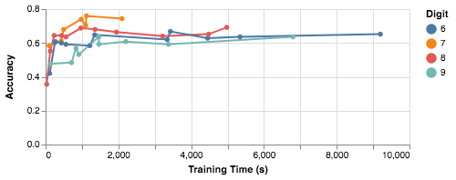
Each training line ends when the synthesizer proves that no better result is possible for the training set—in other words, the final classifier is the optimal one for the given training data. The test-set accuracy is better than random in all four cases, which is a big improvement over our first effort, and some classifiers get over 75% accuracy. Most impressively to me, the synthesis time is much lower than the original 7 days—all four digit classifiers get close to their best accuracy after about 15 minutes (that’s pretty good by synthesis standards!).

What did we learn?

Training a neural network with an SMT solver is a very bad idea. The takeaway from this work isn’t that we should throw out TensorFlow and replace it with a synthesis-based pipeline—75% accuracy on MNIST is unlikely to win us any best paper awards. What’s interesting about these results is that the tools we’re using were never designed with anything like this in mind, and yet (with a little fine-tuning) we can get some credible results. The problem that ends up dooming our approach is training data: our synthesizer needs to see all the training data upfront, encoded as assertions, and this quickly leads to intractable problem sizes.

I think there are two exciting future directions that can skirt around this problem. One is to focus more on verification, as Reluplex does. The fact that we can get any results at all for this synthesis problem bodes well for verification, which tends to be easier for automated tools (one way to think about it is that synthesis quantifies over all neural networks, whereas verification cares only about a single network). Our synthesis infrastructure even allows us to prove negative results, as in our XOR experiments.

The second direction is to use synthesis techniques to augment machine learning. There are some exciting early results in using synthesis to generate interpretable programs to describe the behavior of a black-box neural network. Given a trained black-box network, there’s no need for the synthesis phase to see all the training data, which helps avoid the scaling issues we saw earlier. This approach combines the strengths of both synthesis and machine learning.

We’re omitting bias terms from our neural network implementation, but they would be easy to add. ↩
The (let loop ([a b]) expr ...) form in this code is defining and immediately invoking a recursive function; it’s equivalent to (letrec ([loop (lambda (a) expr ...)]) (loop b)). ↩