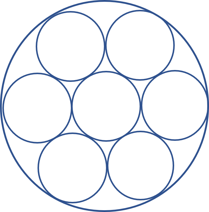
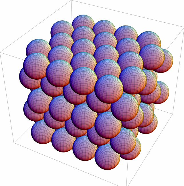
Curse of dimensionality
In $\mathbb{R}^k$, volumes grow polynomially in the dimension: The volume of the Euclidean ball $\{ x \in \mathbb{R}^k : |x| \leq r \}$ of radius $r$ is proportional to $r^k$. One consequence of this is that one can pack $c^k$ disjoint balls of radius $r$ inside a ball of radius $2r$, for some $c > 1$.
Dimension reduction
One straightforward way of coping with the curse of dimensionality is by reducing the dimension of a dataset. Here is a famous lemma of Johnson and Lindenstrauss.
We will define a random $d \times k$ matrix $\mathbf{A}$ as follows. Let \(\{X_{ij} : 1 \leq i \leq d, 1 \leq j \leq k \}\) denote a family of independent $N(0,1)$ random variables. We define
\[\mathbf{A}_{ij} = \frac{1}{\sqrt{d}} X_{ij}\]JL Lemma: Consider \(n \geq 1\) and \(\varepsilon > 0\). Let \(d = \lceil \frac{24 \ln n}{\varepsilon^2}\rceil\). Then for the random map \(\mathbf{A} : \mathbb{R}^k \to \mathbb{R}^d\) defined above and any $n$-point subset $X \subseteq \mathbb{R}^k$, with probability close to one it holds that for all $x,y \in X$:
In other words, by taking a random matrix mapping \(d\) dimensions to \(O(\log n)\) dimensions, one will (with high probability) preserve all interpoint distances for any given set of $n$ points. In fact, it turns out that many such matrices will do the trick. One could also take the entries \(\mathbf{A}_{ij} \in \{-1,1\}\) to be independent random signs.
A formal proof of this lemma can be found in the CSE 525 lecture notes. The basic idea is to define a random one-dimensional map \(\mathbf{F} : \mathbb{R}^k \to \mathbb{R}\) that maintains some of the distance information (in expectation), and then (like in our previous work on hashing) to concatenate $d$ independent such maps and use the power of independence to prove that we can (approximately) preserve many interpoint distances simultaneously.
Locality-sensitive hashing
We will come back to the construction of the random one-dimensional map for the JL lemma later. Let us first see some other examples of hash functions that approximately preserve similarity.
MinHash
Recall the Jaccard similarity. Suppose that \(U\) is the set of all movies available on Netflix and we represent a pair of users \(A,B \subseteq U\) as sets of the movies they have watched. The Jaccard similarity between \(A\) and \(B\) is
\[J(A,B) = \frac{|A \cap B|}{|A \cup B|}\,.\]We define a hash function as follows. Assume, for simplicity, that \(U = \{ 1,2,\ldots,n \}\). We first choose a random permutation $\pi : U \to U$, and then for a user $S \subseteq U$, we define
\[h_{\pi}(S) = \mathrm{argmin}_{x \in S} \pi(x)\,.\]In other words, if we think of $\pi$ as a random labeling of the movies $U$, then $h_{\pi}(S)$ is the element of $S$ with the smallest label.
A cool fact is that the probability of two users colliding under this random hash function is precisely their similarity $J(A,B)$:
\[\Pr[h_{\pi}(A)=h_{\pi}(B)] = \frac{|A \cap B|}{|A \cup B|} = J(A,B)\,.\]To see this, let \(\mathbf{z}\) denote the element of \(A \cup B\) that \(\pi\) gives the smallest label. If \(\mathbf{z} \in A \setminus B\) then \(h_{\pi}(A) = \mathbf{z}\), but \(h_{\pi}(B) \neq \mathbf{z}\). Symmetrically, the hashes are also different if \(\mathbf{z} \in B \setminus A\). But if \(\mathbf{z} \in A \cap B\), then \(h_{\pi}(A)=\mathbf{z}=h_{\pi}(B)\). Therefore:
\[\Pr[h_{\pi}(A)=h_{\pi}(B)] = \Pr[\mathbf{z} \in A \cap B] = \frac{|A \cap B|}{|A \cup B|}\,.\]Using independence
Suppose we choose \(\ell\) hash functions \(h_1,h_2,\ldots,h_{\ell}\) independently from this distribution and define the $\ell$-dimensional hash
\[H(S) = (h_1(S),\ldots,h_{\ell}(S)).\]And define the dimension-reduced similarity:
\[J^H(A,B) = \frac{\# \{ i : h_i(A)=h_i(B) \} }{\ell}.\]This is the fraction of times that users $A$ and $B$ have the same hash value.
It is not too hard to show that for \(\ell \leq O\left(\frac{\log n}{\varepsilon^2}\right)\), for any set \(X\) of \(n\) users, the following holds with high probability:
\[(1-\varepsilon) J(A,B) \leq J^H(A,B) \leq (1+\varepsilon) J(A,B)\,.\]One might compare this to the statement of the JL lemma.
Nearest-neighbor search
Locality-sensitive hashing schemes can be used to build data structure for nearest-neighbor search in high dimensions. A good overview appears in this homework assignment from CSE 525.
The basic idea is that if similar elements often hash into the same bucket, then one can precompute an $\ell$-dimensional vector of hashes
\[H(x) = \left(h_1(x),\ldots,h_{\ell}(x)\right)\]for all the elements \(x \in \mathcal{D}\) in the database. Now when a query $q$ comes, one can compute \(H(q)\) and look for the closest point from \(\mathcal{D}\) by checking all those points \(x \in \mathcal{D}\) that have \(H(x)=H(q)\).
If the hash family additionally has the property that far away points tend to hash to different buckets, then we might expect that the number of points in the same bucket as $q$ is relatively small, and thus we can check this bucket by brute force (or by using a slower search algorithm).
The one-dimensional JL hash
Returning to the JL-lemma, we will define our one-dimensional hash as follows: For a vector \(r \in \mathbb{R}^k\), define the map \(F_r : \mathbb{R}^k \to \mathbb{R}\) by
\[F_r(x) = \langle x, r\rangle = x_1 r_1 + x_2 r_2 + \cdots + x_k r_k\]In other words, we map \(k\) dimensions to 1 dimension by projecting onto the direction \(r\).
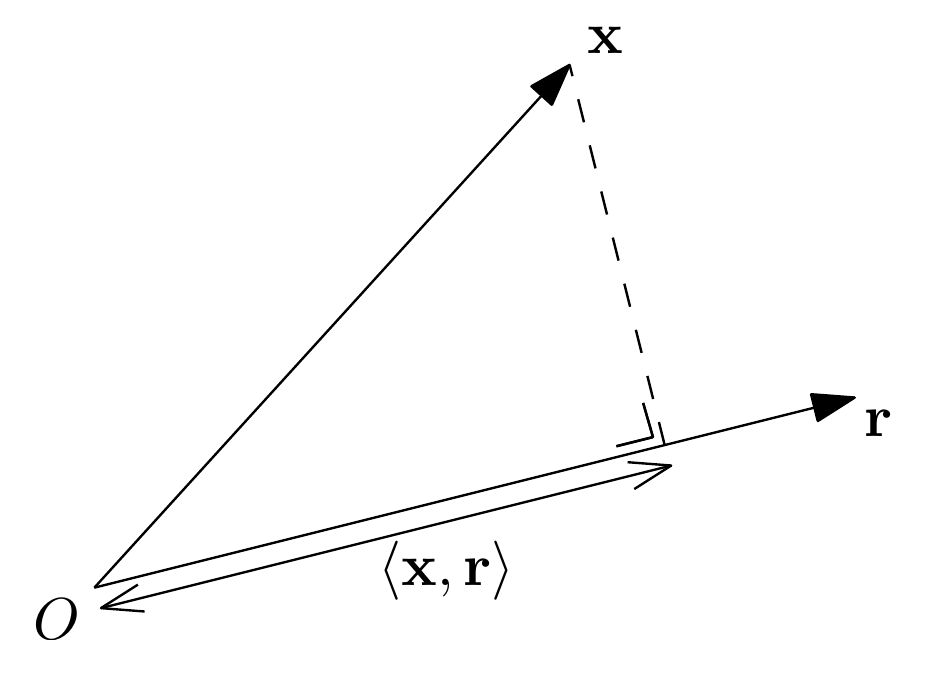
We will choose \(\mathbf{r} = (r_1,r_2,\ldots,r_k)\) to be a random direction specified by choosing each $r_i$ to be an independent \(N(0,1)\) random variable.
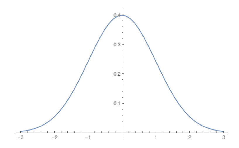
Recall from CSE 312 that the normal distribution is determined by its mean \(\mu\) and
variance \(\sigma^2\). The standard normal distribution has \(\mu=0\)
and \(\sigma = \sigma^2 = 1\). Here is the density function for an $N(0,1)$
random variable:
Two stability
A key property of normal random variables is that they are 2-stable. This means that if \(X_1\) and $X_2$ are independent random variables with normal distributions \(N(\mu_1,\sigma_1^2)\) and \(N(\mu_2,\sigma_2^2)\), then \(X_1+X_2\) has the distribution of an \(N(\mu_1+\mu_2, \sigma_1^2+\sigma_2^2)\) random variable. Note that it’s not surprising that the means add (this is linearity of expectation) and it’s not surprising that the variances add (this is true for any pair of independent random variables). The interesting property is that the resulting distribution is again normal.
For instance, if \(X_1\) and \(X_2\) are independent random variables uniformly distribution on \([0,1]\), then \(X_1+X_2\) is certainly not uniform on \([0,2]\).
Returning to our one-dimensional hash \(F_{\mathbf{r}}(x) = \langle x,\mathbf{r}\rangle\), since the coordinates \(r_1,\ldots,r_k\) are independent \(N(0,1)\) random variables, the two stability property tells us that for any \(x \in \mathbb{R}^k\), the random variable \(\langle x,\mathbf{r}\rangle = x_1 r_1 + x_2 r_2 + \cdots + x_k r_k\) has mean zero and variance
\[x_1^2 + x_2^2 + \cdots + x_k^2 = \|x\|_2^2\]That’s because each summand \(x_i r_i\) is an \(N(0, x_i^2)\) random variable.
So this random inner product is an “unbiased estimator” for the squared Euclidean length of the vector \(x\):
\[\mathbb E[F_{\mathbf{r}}(x)^2] = \mathbb E[\langle x,\mathbf{r}\rangle^2] = \|x\|_2^2\,.\]Since the inner product is linear, we actually get something for any pair of vectors \(x,y\in \mathbb{R}^k\):
\[\mathbb E[(F_{\mathbf{r}}(x)-F_{\mathbf{r}}(y))^2] = \mathbb E[(\langle x, \mathbf{r}\rangle - \langle y,\mathbf{r}\rangle)^2] = \mathbb E[\langle x-y, \mathbf{r}\rangle^2] = \|x-y\|_2^2\]Just as in the sketch for MinHash, the JL Lemma is now proved by doing this many times independently, i.e., by choosing \(d\) random directions \(\mathbf{r}_1, \mathbf{r}_2, \ldots, \mathbf{r}_d \in \mathbb{R}^k\) and taking the final mapping
\[x \mapsto \frac{1}{\sqrt{d}} \left(F_{\mathbf r_1}(x), F_{\mathbf r_2}(x), \ldots, F_{\mathbf r_d}(x)\right) = \frac{1}{\sqrt{d}} \left(\langle x,\mathbf r_1\rangle, \langle x,\mathbf r_2\rangle, \ldots, \langle x,\mathbf r_d\rangle\right)\]This mapping is precisely given by \(x \mapsto \mathbf{A} x\) where $\mathbf{A}$ is the random matrix we defined earlier. To see this, note that if \(M\) is a matrix with rows \(m_1, m_2, \ldots, m_d \in \mathbb{R}^k\) and \(x \in \mathbb{R}^k\), then
\[Mx = (\langle x, m_1\rangle, \langle x,m_2\rangle,\ldots,\langle x,m_d\rangle)\](In matrix form, the right-hand side would be a column vector.)