Spectral graph theory is a powerful and beautiful way of understanding graphs by representing them as matrices and then considering the eigenvalues and eigenvectors of those matrices. This leads to many other useful ways of reimaging graphs as physical systems: For instance, as bodies that allow heat to transfer from one region to another, or as electral networks that carry electrons along edges. \(\def\seteq{\mathrel{\vcenter{:}}=} \def\cE{\mathcal{E}} \def\R{\mathbb{R}} \def\argmin{\mathrm{argmin}} \def\llangle{\left\langle} \def\rrangle{\right\rangle} \def\1{\mathbf{1}} \def\e{\varepsilon} \def\avint{\mathop{\,\rlap{-}\!\!\int}\nolimits}\)

Graphs as matrices

We will consider undirected graphs \(G=(V,E)\) without loops or multiple edges. We use \(n = |V|\) to denote the number of vertices. There are many matrices one can associate to such a graph; perhaps the most natural is the \(V \times V\) adjacency matrix defined by

\[A_{uv} = \begin{cases} 1 & \{u,v\} \in E \\ 0 & \textrm{otherwise.} \end{cases}\]

Another extremely useful matrix is the closely related Laplacian matrix defined by \(L_G = D - A\) where \(A\) is the adjacency matrix of \(G\) and \(D\) is the diagonal degree matrix, i.e., with \(D_{vv}=\deg(v)\) and \(D_{uv}=0\) for \(u \neq v\). Equivalently,

\[(L_G)_{u,v} = \begin{cases} \deg(u) & u = v \\ -1 & \{u,v\} \in E \\ 0 & \textrm{otherwise.} \end{cases}\]

Note that both the adjacency matrix and Laplacian are symmetric matrices.

If we write \(L_e\) for the Laplacian of the graph with vertex set \(V\) but only a single edge \(e=\{u,v\}\), then we can build \(L_G\) from these edge graphs:

\[\begin{equation}\label{eq:edge-sum} L_G = \sum_{e \in E} L_e \end{equation}\]

This helps us to apply \(L_G\): If \(\mathbf{x} \in \R^V\), then

\[\begin{equation}\label{eq:diffusion} (L_G \mathbf{x})_u = \sum_{e \in E} (L_e \mathbf{x})_u = \sum_{v : \{u,v\} \in E} (x_u - x_v) \end{equation}\]

In other words, \((L_G \mathbf{x})_u\) is the sum of the changes of \(\mathbf{x}\) along edges out of vertex \(u\).

Aside: Relationship to the Laplacian from calculus

From calculus (or physics) class, you may remember that the Laplace operator is a map that assigns to a (sufficiently nice) function \(f : \R^n \to \R\), the sum of the second-order partial derivatives:

\[\Delta f = \sum_{i=1}^n \frac{\partial^2 f}{\partial x_i^2}\]

There is another more physical way to think about this operator:

\[\begin{equation}\label{eq:sphere} \Delta f(x) = \lim_{r \to 0} \avint_{S_r(x)} \left(f(y)-f(x)\right)\,dy \end{equation}\]

That is, to compute the value at \(x\), we look at the average change in \(f\) over small spheres \(S_r(x)\) about \(x\), and then we take the limit as \(r \to 0\). The reason that the differential form of \(\Delta f\) only has second-order derivatives is that the first order terms cancel out because we average in a spherically symmetric way about \(x\).

If one thinks of \(f\) as assigning a temperature to every point in space, then \(\Delta f(x)\) represents the mean deviation in temperature at \(x\). This leads to the famous heat equation:

\[\frac{\partial h_t(x)}{\partial t} = \Delta h_t(x)\]

that describes the evolution of heat \(h_t(x)\) in space as time evolves.

Similarly, \eqref{eq:diffusion} represents the total deviation of the value \(x_u-x_v\) as we sum over neighbors \(v\) of \(u\) in \(G\) (this is like the “sphere” around \(u\) in \(G\)). For various historical reasons, the sign of the graph Laplacian is the opposite of the sign of the differential Laplace operator (compare to \eqref{eq:sphere}).

The eigenvalues and eigenvectors of \(L_G\)

Building off the expression \eqref{eq:diffusion}, we can compute

\[\begin{equation}\label{eq:qform} \langle \mathbf{x}, L_G \mathbf{x} \rangle = \sum_{\{u,v\} \in E} \langle \mathbf{x}, L_{\{u,v\}} \mathbf{x}\rangle = \sum_{\{u,v\} \in E} (x_u - x_v)^2, \end{equation}\]

where we used for every edge \(\{u,v\} \in E\), the simple calculation

\[\langle \mathbf{x}, L_{\{u,v\}} \mathbf{x}\rangle = x_u (x_u-x_v) + x_v (x_v - x_u) = (x_u-x_v)^2\]

Since \(L_G\) is a real symmetric matrix, all its eigenvalues are real numbers and it has an orthonormal basis of eigenvectors. If \(\mathbf{x}\) is an eigenvector with eigenvalue \(\lambda\), then \(L_G \mathbf{x} = \lambda \mathbf{x}\), hence

\[\begin{equation}\label{eq:lambda} \langle \mathbf{x}, L_G \mathbf{x} \rangle = \lambda \langle \mathbf{x},\mathbf{x}\rangle = \lambda \|x\|^2 \end{equation}\]

The expression \eqref{eq:qform} shows that \(\langle \mathbf{x}, L_G \mathbf{x}\rangle \geq 0\), hence \(\lambda \geq 0\) as well, and we see that all the eigenvalues of \(L_G\) are non-negative. (Such a matrix is called positive semidefinite.)

The zero eigenvalue

Let us order the eigenvalues of \(L_G\) in increasing order \(\lambda_1 \leq \lambda_2 \leq \cdots \leq \lambda_n\). We know that \(\lambda_1 \geq 0\). It turns out that actually \(\lambda_1=0\) as we can see from taking the constant vector \(\mathbf{x}_1 = (1/\sqrt{n},1/\sqrt{n},\ldots,1/\sqrt{n})\). Then \(\lambda_1=0\) follows from \eqref{eq:lambda} using the fact that the value of \eqref{eq:qform} is zero.

Recall that we could have more than one zero eigenvalue. If \(\lambda_1=\lambda_2=\cdots=\lambda_h=0\) and \(\lambda_{h+1} > 0\), one says that the eigenvalue zero has multiplicity \(h\). What is the multiplicity of the zero eigenvalue of \(L_G\)? This gives us our first glimpse that the spectral structure of the Laplacian says something interesting about \(G\).

LEMMA: The multiplicity of the eigenvalue zero in \(L_G\) is precisely the number of connected components in \(G\).

PROOF: Suppose that the vertices of \(G\) are partitioned into \(h\) connected components \(V = S_1 \cup S_2 \cup \cdots \cup S_h\). First, let us show that \(\lambda_1=\lambda_2=\cdots=\lambda_h=0\). We can do this by finding \(h\) orthogonal vectors \(\mathbf{x}_1, \ldots, \mathbf{x}_h\) such that \(L_G \mathbf{x}_0 = L_G \mathbf{x}_1 = \cdots = L_G \mathbf{x}_h = 0\).

Define: \(\mathbf{x}_i(u) = 1\) if \(u \in S_i\) and \(\mathbf{x}_i(u) = 0\) otherwise. Then \eqref{eq:qform} shows that \(\langle \mathbf{x}_i, L_G \mathbf{x}_i\rangle = 0\) for each \(i=1,2,\ldots,h\) because each vector \(\mathbf{x}_i\) is constant on connected components. Moreover, \(\langle \mathbf{x}_i, \mathbf{x}_j\rangle = 0\) for every \(i \neq j\) because the vectors have disjoint supports (they are non-zero on disjoint sets of coordinates).

Now let us argue that if \(G\) has exactly \(h\) connected components, then \(\lambda_{h+1} > 0\). Suppose that \(\mathbf{x}\) is orthogonal to the vectors \(\mathbf{x}_1,\ldots,\mathbf{x}_h\) we defined above and that \(\langle \mathbf{x}, L_G \mathbf{x}\rangle = 0\). Using \eqref{eq:qform} again, the second fact implies that \(\mathbf{x}\) is constant on connected components. Moreover, since \(\mathbf{x} \neq (0,\ldots,0)\), it must be that \(\mathbf{x}(u) = c\neq 0\) for some \(u\). If \(u \in S_i\), then \(\mathbf{x}(v) = c\) for all \(v \in S_i\), which means that \(\mathbf{x}\) and \(\mathbf{x}_i\) cannot be orthogonal.

Higher eigenvalues and eigenvectors

To understand various eigenvectors, it helps to think of an eigenvector \(\mathbf{x} \in \R^V\) as assigning a label \(\mathbf{x}_u\) to every vertex \(u \in V\). The low eigenvectors are those that minimize the quadratic form

\[\langle \mathbf{x}, L_G \mathbf{x}\rangle = \sum_{\{u,v\} \in E} ({x}_u - {x}_v)^2,\]

i.e., those that assign labels to vertices so that the endpoints of edges have similar labels. Obviously this expression is minimized by choosing a vector \(\mathbf{x}\) that is constant on connected components (in which case it has value zero).

The variational formula for eigenvalues says that the second eigenvalue is given by

\[\lambda_2 = \min \left\{ \sum_{\{u,v\} \in E} ({x}_u - {x}_v)^2 : \mathbf{x} \perp \mathbf{x}_1 \textrm{ and } \|\mathbf{x}\| = 1\right\},\]

where \(\mathbf{x}_1\) is the first eigenvector. The second eigenvector is the corresponding minimizer. Similarly, one has the formula

\[\begin{equation}\label{eq:variational} \lambda_k = \min \left\{ \sum_{\{u,v\} \in E} ({x}_u - {x}_v)^2 : \mathbf{x} \perp \mathbf{x}_1, \ldots, \mathbf{x} \perp \mathbf{x}_{k-1} \textrm{ and } \|\mathbf{x}\| = 1\right\}, \end{equation}\]

where \(\mathbf{x}_1,\ldots,\mathbf{x}_{k-1}\) are the first \(k-1\) eigenvectors.

The highest eigenvectors (again, we mean those associated to the largest eigenvalues) tend to maximize the this quantity. Indeed, the variational formula also implies that

\[\lambda_n = \max \left\{ \sum_{\{u,v\} \in E} ({x}_u - {x}_v)^2 : \|\mathbf{x}\| = 1\right\},\]

and the analog of \eqref{eq:variational} holds for \(\lambda_{n-1}, \lambda_{n-2}\), etc.

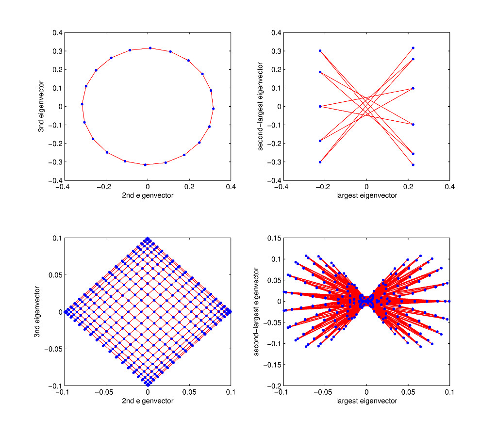
This intuition is confirmed in the spectral embedding pictures below.

Some applications of spectral graph theory

Visualizing a graph and spectral embeddings

The non-zero eigenvalues (and associated eigenvectors) often contain very interesting information about \(G\). For instance, here are embeddings of the cycle and grid graphs using the small eigenvectors (corresponding to the second and third eigenvalues) as well as the large eigenvectors (corresponding to the largest and second-largest eigenvalues).

An eigenvector \(\mathbf{x}\) assigns real numbers \(\mathbf{x}(u)\) to the vertices \(u \in V\). If we use two such eigenvectors, we get a two-dimensional representation of the graph. For instance, in the embedding of a cycle on \(20\) vertices, we map every vertex \(u \in V\) to the point \((\mathbf{x}_2(u), \mathbf{x}_3(u))\) where \(\mathbf{x}_2\) and \(\mathbf{x}_3\) are the second and third smallest eigenvectors.

These pictures confirm our intuition that the small eigenvectors tend to make edges “short” while the large eigenvectors tend to map the endpoints of edges far apart.

Spectral clusering

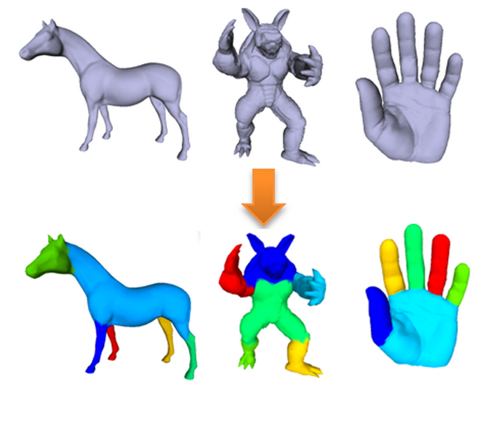
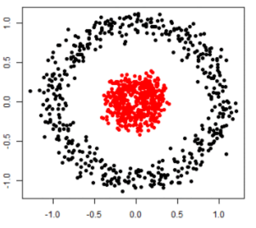
As we will see more formally in the next lecture, eigenvectors can be used to identify meaningful clusters in data represented as graphs. Such clusters can be especially “hidden” in very large networks (e.g., social networks or protein interactions).

In this video, one can observe the simulation of a virus infecting users in a network, and it is unclear what distinguishes infected nodes from uninfected ones. In this video, the network is embedded along the second eigenvector, revealing that the network is formed from two densely connected clusters that are only sparsely connected to each other.

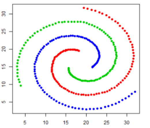
Further eigenvectors can be used to find more clusters. And spectral clustering has the ability to locate non-linear patterns in a data set.

Graph coloring

Consider the motivating example of allocating one of \(k\) different radio bandwidths to each radio station. If two radio stations have overlapping regions of broadcast, then they cannot be assigned the same bandwidth (otherwise there will be interference for some listeners). On the other hand, if two stations are very far apart, they can broadcast on the same bandwidth without worrying about interference from each other. This problem can be modeled as the problem of \(k\)-coloring a graph. In this case, the nodes of the graph represent radio stations, and there is an edge between two stations if their broadcast ranges overlap. The problem then, is to assign one of \(k\) colors (i.e., one of \(k\) broadcast frequencies) to each vertex, such that no two adjacent vertices have the same color. This problem arises in several other contexts, including various scheduling tasks (in which, for example, tasks are mapped to processes, and edges connect tasks that cannot be performed simultaneously).

This problem of finding a \(k\)-coloring, or even deciding whether a \(k\)-coloring of a graph exists, is NP-hard in general. One natural heuristic, which is motivated by the right column of the spectral embeddings above, is to embed the graph onto the eigenvectors corresponding to the highest eigenvalues. Recall that these eigenvectors are trying to make vertices as different from their neighbors as possible. As one would expect, in these embeddings, points that are close together in the embedding tend to not be neighbors in the original graph.

Hence one might imagine a \(k\)-coloring heuristic as follows: 1) plot the embedding of the graph onto the top 2 or 3 eigenvectors of the Laplacian, and 2) locally partition the points in this space into \(k\) regions, e.g., using \(k\)-means, or a kd-tree, and 3) assign all the points in each region the same color. Since neighbors in the graph will tend to be far apart in the embeddings, this tends to give a decent coloring of the graph. There are semidefinite programming algorithms based on a generalization of this idea that are able to (provably) color graphs with a small number of colors.