Problem 1: Markov chains

For each of the following three graphs, consider a Markov chain defined by a random walk over the nodes of the graph:

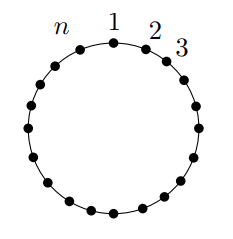
1. The cycle graph with \(n=13\).
2. The cycle graph with \(n=12\).
3. The cycle graph with \(n=13\) and an extra edge connecting nodes $1$ and $6$.

(a) [2 points]

For each Markov chain, explain whether it is aperiodic or irreducible. If it is aperiodic and irreducible, what is its stationary distribution?

(b) [4 points]

Given a Markov chain and an initial state $s$, let \(\mu_v(t)\) denote the distribution of the state after \(t\) transitions of the chain starting the random walk from \(v\).

Take \(v=1\) and for each of the three chains, plot \(\|\mu_v(t)-\pi\|_{TV}\) for \(t \in \{0,1,2,\ldots,100\}\), where the total variation distance between two distributions \(p_1\) and \(p_2\) on a domain \(\Omega\) is defined as

\[\|p_1-p_2\|_{TV} = \frac12 \sum_{v \in \Omega} |p_1(v)-p_2(v)|.\]

Graph the three lines on the same plot, clearly labeling them. For the Markov chains that are not both aperiodic and irreducible, set \(\pi\) to be equal to the uniform distribution in your total variation calculations.

Include both a plot and your code for this part.

(c) [2 points]

Report the values of the second-largest eigenvalue of the transition matrix for each of these three Markov chains.

(d) [5 points]

Discuss the results of parts (b) and (c) and their connection. You should specifically mention the mixing time and the power iteration algorithm. You could also explore additional graphs (e.g., where you add more edges) to investigate the relation between the mixing time and the second-largest eigenvalue.

Problem 2: Visiting 30 national parks

Your goal is to design a short tour of 30 national parks. This is a route starting from one park, visiting all the parks in some order, and the returning to the starting point. In the file parks.csv, you’ll find the longitude and latitude of the 30 national parks in alphabetical order (by the park name).

To simplify the problem, you may assume that the distance between two national parks is given by the distance

\[\textrm{distance} = \sqrt{(\textrm{longitude}_1 - \textrm{longitude}_2)^2 + (\textrm{latitude}_1 - \textrm{latitude}_2)^2}\]

To make sure your distance calculation is correct, the distance between Acadia and Arches (the first two listed in the file) is \(41.75\) units, and the total length of the tour that visits all the parks in alphabetical order and then returns to Acadia is \(491.92\).

You will now study an MCMC algorithm that is parameterized by a “temperature” parameter \(T\) that governs the tradeoff between local search and random search. The algorithm is as follows.

• Start with a uniformly random permutation of the \(N=30\) parks. This is your initial tour \(\tau\).

• For \(i=1,2,\ldots,\tt{NUMITER}\):

  • Choose a uniformly random pair of consecutive parks in your current tour \(\tau\). Let \(\tau'\) be the tour that results from switching the order of those two parks.

  • If \(\tau'\) has lower total length than the current tour \(\tau\), set \(\tau := \tau'\).

  • Otherwise, if \(T > 0\), with probability \(e^{-\Delta_d/T}\), update \(\tau := \tau'\), where \(\Delta_d = \textrm{length}(\tau') - \textrm{length}(\tau)\) is the difference in total length between \(\tau'\) and \(\tau\).

(a) [2 points]

Implement the MCMC algorithm. Have your algorithm also keep track of the best tour seen during all NUMITER iterations. Include your code.

How many states are in your Markov chain? If the number of iterations tends to infinity, would you eventually see all possible routes?

(b) [4 points]

Set NUMITER to be 12,000. Run the algorithm in four different regimes, with \(T \in \{0,1,10,100\}\). For each value of \(T\), run \(10\) trials. Produce one figure for each value of \(T\). In each figure, plot the line for each trial: The iteration number against the length of the current route \(\tau\) of the route (not the current value of the best tour seen so far) during that iteration. (Your solution will contain 4 figures, end each plot should have 10 lines.) Among the 4 value of \(T\), which one seems to work the best?

(c) [2 points]

Modify the above MCMC algorithm as follows: In each iteration, select two parks completely at random (as opposed to two consecutive parks in \(\tau\)). Repeat the experiments for part (b). Among the 4 values of \(T\), which one seems to work the best now?

(d) [4 points]

Describe whatever differences you see relative to part (b), and propose an explanation of why this Markov chain performs differently than the previous one. If the best values of \(T\) are different in the two parts, try to provide an explanation. (You may wish to think about this problem relative to your investigation of the mixing times of different Markov chains in Problem 1.)

Problem 3 (Extra credit): Chebyshev

Recall Chebyshev’s inequality: For every random variable \(X\) and number \(\lambda > 0\), it holds that

\[\Pr\left[|X-\mathbb{E}[X]| \geq \lambda \right] \leq \frac{\mathrm{Var}(X)}{\lambda^2}\]

Your goal in this problem is to prove the following: For any \(n\) real numbers \(a_1,a_2,\ldots,a_n\) satisfying \(a_1^2 + a_2^2 + \cdots + a_n^2 = 1\), if \(\sigma_1,\sigma_2,\ldots,\sigma_n \in \{-1,1\}\) are i.i.d. uniform random signs, then

\[\Pr\left[\left|\sum_{i=1}^n \sigma_i a_i\right| \leq 1\right] \geq \frac{1}{32}.\]

(a) [5 points] Case I: A big coefficient

For simplicity, we may sort so that \(\lvert a_1\rvert \geq \lvert a_2 \rvert \geq \cdots \geq \lvert a_n\rvert\). Define \(X = \sum_{i=1}^n a_i \sigma_i\). Assume now that \(\lvert a_1\rvert \geq 1/\sqrt{2}\). Apply Chebyshev’s inequality to the random variable \(X_1 = X - a_1 \sigma_1\) to conclude that

\[\Pr[\lvert X\rvert \leq 1] \geq 1/4.\]

(b) [10 points] Case II: All small coefficients

Now assume that \(1/\sqrt{2} > \lvert a_1\rvert \geq \lvert a_2\rvert \geq\ldots \geq \lvert a_n\rvert\).

Split the sum \(X = Y+Z\) into two pieces (hint: try to choose them to be “balanced”) and apply Chebyshev’s inequality separately to \(Y\) and \(Z\) to conclude that \(\Pr[\lvert X\rvert \leq 1] \geq \frac{1}{32}\) in this case as well.