
Introduction to Statistical and Computational Genomics
GENOME 559Department of Genome Sciences
University of Washington School of Medicine
Homework 7
Due: 3/16
Notes: Again, please track your hours, and report them here (not quite anonymously).
Electronic Turnin: Please turn in hw7.py, plus any
necessary Python module files you might have chosen to
create: here.
Include any extra credit file(s) with "-ec" added to the file name,
e.g., hw7-ec.py.
The short "written" portion of the assignment may be turned in on
paper in class, to Ruzzo's office, or electronically.
Problems:
We will reuse the GenBank record for the M. jannaschii genome that you downloaded for homework 5. (Fetch it again, if you didn't happen to save it.) The plan is to again find its tRNAs, but using Biopython to do nearly all of the work. (In particular, there's little, if any, from HW 5 that you'll be able to reuse, but hopefully seeing it done two ways will be interesting.) My solution is about two dozen lines long, half print statements (excluding comments). Yours may of course be longer, but if it's growing much more complex than that, you might want to review your approach. Your main challenge (I think) will be navigating through the Biopython libraries and its SeqRecord class to find the parts you need. My slides, the Biopython Tutorial & Cookbook (esp. sections 2.4 / 2.4.2, 4.1, 13 / 13.1 / 13.1.2, with special emphasis on "nofuzzy") and direct experimentation using python (help(), type(), dir(), ...) should give you what you need.
If needed, download and install Biopython.
Read and "parse" the .gbk file using the appropriate SeqIO function. All of the following information including the full nucleotide sequence is directly available or easily calculated from data in the SeqRecord object; you shouldn't need to look at the .gbk file in any other way.
Using the annotations and "feature table" built by SeqIO, print the (i) record description, (ii) ID, (iii) genome length and (iv) the genome-wide GC %.
Then find and print (i) the genomic coordinates, (ii) length, (iii) strand and (iv) GC % for each tRNA.
    Description: Methanocaldococcus jannaschii DSM 2661, complete genome.
    ID: NC_000909.1 , Length: 1664970 , GC: 31%
    37 Annotated tRNAs:
     #   Start..    End Len Strand GC%
     1   97428..  97537 109     -1 62%
     2   97628..  97713  85      1 67%
     3  111767.. 111852  85      1 73%
    ...
    37 1313164..1313249  85      1 73%
Notes: Be careful about coordinates. E.g., GenBank records use 1-based indexing of nucleotides (i.e., start numbering the nucleotides from 1), whereas Python uses zero-based indexing. Are the coordinates in the Biopython feature table 0-based or 1-based? Is the "end" coordinate the last nucleotide of the feature or the one after the last?
In the pedigree at right,
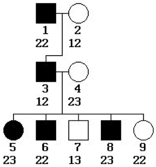
- Does the phenotype being tracked appear to be sex-linked or autosomal? Explain.
- Dominant or recessive? Explain.
- How many non-recombinant and recombinant offspring are there? Explain.
- What value of the recombination rate θ would you estimate from this data?
- What is the LOD score for linkage between the phenotype and the typed locus? Is it significant?
Extra Credit Ideas: Instead of using your web browser to fetch the M. jannaschii genome from GenBank, get it via the Biopython interface to NCBI's "EFetch" utility. To save yourself a lot of time, and to avoid burdening NCBI's servers with repeated fetches as you debug, have your code "cache" a copy on your hard drive, re-fetching it only if that copy is not found; see section 7 / 7.6 / 7.11 of the Biopython tutorial for an example of how to do this, be sure to note the code related to "os.path.isfile()" and be sure to read 7.1 "Entrez Guidelines"