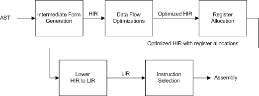
Figure 1. Optimizing compiler backend.
The diagram below shows a high-level design for the back end of an optimizing compiler, so you can see where register allocation fits in. Specifically, this shows how the backend translates the AST for one procedure into optimized assembly code.

Figure 1. Optimizing compiler backend.
These notes present the graph coloring method of register allocation. This method produces better code than previous methods and is used in most optimizing compilers.
The diagram below shows the main steps of the basic register allocation algorithm. We will explain the steps along with an example.
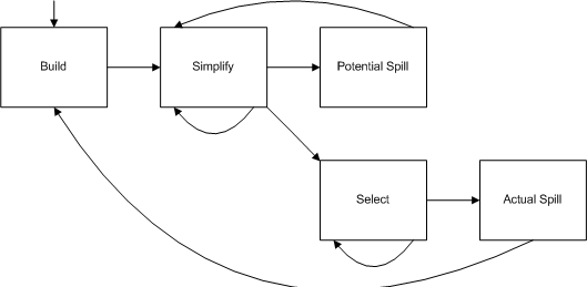
Figure 2. Register allocation algorithm.
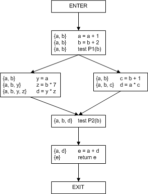
Figure 3. Example CFG.
Build the register interference graph (RIG). First, we need the set of live variables at each program point. This is shown in the CFG and is computed by solving the live-variables data-flow analysis problem. Next, we create a graph with a node for each variable, and edges connecting registers that are live at the same time.
The RIG tells us which variables cannot share registers, because two distinct variables that are simultaneously live cannot share a register. If we have k registers available, our goal is to k-color the graph, because a k-coloring is equivalent to a valid register assignment for every variable.
Here is our RIG. We will assume we have 3 registers available, named r1, r2, and r3.
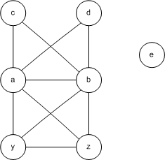
Remove any node with fewer than k siblings and place it on a stack.
This is the coloring heuristic. The idea is that if, by some magic (i.e., the rest of the algorithm), we can k-color the rest of the graph, then we can easily color the whole graph. That's because this node has at most k-1 siblings, so there will be at least one color left over for this node.
We repeat simplify as long as we can keep doing it. If we reach an empty graph, we go on to the select step. If we reach a nonempty graph that cannot be simplified, we go to potential spill.
Here is our RIG after one simplify step.
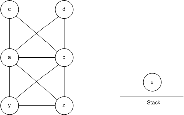
Here is our RIG after a few more simplify steps. After this, we'll go to potential spill.
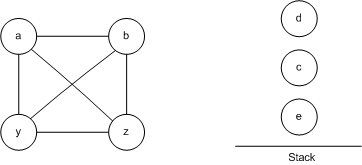
Remove any node and place it on the stack. Then go back to simplify.
This is the optimistic heuristic. This time, we are removing a node with at least k siblings. Even if we can k-color the rest of the graph, we won't necessarily be able to color the whole graph. If this node ends up with a sibling of each of the k colors, we cannot assign it a color. On the other hand, we might be lucky and find that not all k colors are used by the siblings, in which case we would be able to color the graph. So, optimistically, we hope for that case and continue.
Here is our RIG after potential spill.
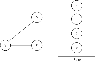
Then we go back to simplify, eventually reaching the following graph, which sends us to select.
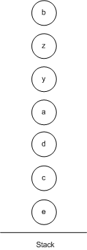
Remove the top node from the stack and add it back to the RIG. Assign the node any color that is not used by any neighbor and repeat select. If there is no such color, go to actual spill.
If the stack is empty, we have successfully assigned registers to all variables and we are done.
This step is the counterpart of simplify or potential spill. When we reach this step, we have k-colored some part of the graph, and we are, if possible, adding a node back and k-coloring the resulting graph.
Here is our RIG after select.
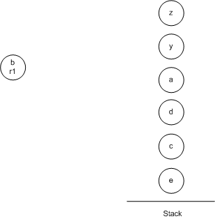
We repeat select, reaching this uncolorable graph, so we go to actual spill.
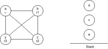
The uncolorable node found by select must be spilled to memory. Assign it a memory location (usually a slot in the activation record). Insert code into the CFG to load it before every use and store it after every definition. Go to build.
We get to this step when the optimistic heuristic failed. Note that this does not necessarily mean there is no k-coloring. It just means that our heuristics didn't find one. Either way, we can't find a k-coloring. So we spill the uncolorable node to memory. This will reduce the number of registers needed, making it more likely we can color the resulting graph.
Here is our CFG after actual spill. Note that we replaced a very large live range for 'a' with smaller live ranges for 't1', 't2', 't3', 't4', and 't5'. This helps us in two ways. First, the combined range covered by these variables is smaller, so there are fewer chances with conflicts. Second, the live range is split up into 5 live ranges, so the conflicts are spread out among more variables, reducing the number of nodes with more than k neighbors.
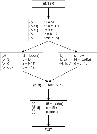
After this, we return to build and basically start over. This is left as an exercise.
This is optional material. This is a list of various refinements to the basic register allocation algorithm. It may be useful in projects. You could use any or all of these ideas in a register allocator.
Consider this code:
a = x + y    // a1

b = x + a    // a1

a = -b       // a2

c = a + 1    // a2
The variable 'a' appears in all four lines, but really there are two separate 'a' variables. There is really no need to use the same register for 'a' on the lines marked 'a1' as on the lines marked 'a2', because the values are not communicated between those lines. And it would be nice to consider them as two nodes in the RIG, because the separate nodes will probably have fewer neighbors than the single node.
The solution is to use webs instead of variables as graph nodes. A web is a set of definitions and uses connected by def-use edges. Variable occurrences in the same web can potentially communicate, so we do want them to get the same register. However, occurrences in two separate webs are completely independent.
To form a web, choose any definition, and find all places where it can be used. Then find all the places those uses can be defined. Continue expanding the web until all the connected instances are in the web. Keep forming webs from variable defs or uses not yet part of a web until all the webs are found.
This affects only the build step. Otherwise, the algorithm is the same, except that it uses webs everywhere the basic algorithm uses variables.
In the basic algorithm, variables interfere if their live ranges overlap at any point. Surprisingly, this constraint is stronger than it needs to be. Consider this CFG, which can happen if there are two ifs with the same test condition and some code in between.
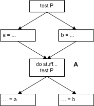
In the block labeled A, both variables a and b are live. However, they do not interfere. (Try to find a code path where you'd get a wrong answer by putting them in the same register. It works even if the test conditions are different.)
Thus, we can get better interference graphs with a more refined condition. The condition is:
Variables 'a' and 'b' interfere if 'a' is live at a point where 'b' is defined (and vice versa).
The intuition is that if 'a' is live where 'b' is defined, we would not want the definition of 'b' to clobber 'a', so we put them in separate registers. On the other hand, if 'a' and 'b' are live together but the live ranges don't overlap definition points, we can only have reached a definition point for one of the two. The other was never defined, so it has a junk value that we don't care about.
Look back at the original CFG, at the statement "y = a". If we could assign the same register to 'a' and 'y', then we wouldn't need this statement, and we could remove it as an optimization. This is called register coalescing.
You might object that copy propagation would have removed this statement in a real compiler. This is true, but there are other statements like this that are harder to remove in the optimization phase. They tend to arise especially when certain values must be assigned certain fixed registers. Coalescing is definitely a powerful register allocation trick, especially when combined with some the other ideas here.
Coalescing requires several changes to the basic algorithm. First, in
build, we use a second kind of edge that connects
copy-related nodes. For each copy statement a = b
in the program, we add a copy-related edge between 'a' and 'b'. In the
rest of the algorithm, our goal will be to coalesce pairs of
copy-related nodes.
In the original simplify, we removed any node with fewer than k neighbors (assuming k available registers). Now, we will be stricter, and we will remove any node with fewer than k "regular" neighbors and no copy-related neighbors. The reason will become clear in future steps.
When simplify fails to find a removable node, instead of going to potential spill, we go to a new step, called coalesce. In this step we choose two copy-related nodes and combine them into a single node. The neighbor set of the new node is the union of the neighbor set of both original nodes. The new node also carries the variable names of both original nodes. This allows us to allocate a single register to all variables in the combined node, and to remember which nodes have been coalesced, so we can remove the variables. After coalesce, we go back to simplify.
We now have a problem. In general, our algorithm works well when nodes have few neighbors. However, coalesced nodes tend to have many neighbors, which might cause a spill. Spills are very expensive since they go to memory, so we'd prefer to give up on coalescing and accept an extra register copy rather than spilling.
We can handle this with a restriction on which nodes to coalesce. Specifically, we coalesce two nodes only if the new node has fewer than k neighbors of degree greater than or equal to k. If we follow this criterion, then the graph after coalescing will be colorable as long as the original was colorable. To see why, think about what simplify will do next. It will remove all the nodes of degree fewer than k, leaving the combined node with fewer than k neighbors total. Then, it will be able to remove the combined node. So coalescing will not introduce any new uncolorable nodes with this restriction.
This also explains why we simplify before coalescing. Our restriction means we're more likely to be able to coalesce nodes after removing some of the nodes, so we simplify first. And that means simplify should leave copy-related nodes alone, so that they can be coalesced when we're ready to do it.
Recall that when simplify fails, we go to coalesce. What if coalesce can't find a pair of nodes? Then we go to freeze, which looks for a copy-related node of degree less than k and removes all of its copy-related edges and go to simplify. We know we can't safely coalesce it, but we will be able to simplify it.
If freeze fails to find a node, we have nothing left to try, so we go to potential spill.
For complete information on coalescing, see Iterated Register Coalescing by George and Appel.
Sometimes there are variables that must be assigned to certain specific registers. For example, on IA-32, the return value goes into $eax. This could be implemented in the code generator. It can also be done in the register allocator using precoloring.
First, we modify the IR to expose the variable if necessary. Thus, the code
a = b + c

return a
turns into
a = b + c

ret {precolor=$eax} = a
The notation {precolor=$eax} represents some kind of
annotation made to the IR indicating that the variable 'ret' must be
assigned $eax. To handle this in register allocation, we add nodes to
the register interference graph for each architectural register: $eax,
$ebx, and so on. For precolored nodes such as 'ret', we add edges to
make them interfere with every architectural register except
the precolor. This indicates that 'ret' cannot get the same color as
$ebx, $ecx, etc., so it can only get the same color as $eax, namely
$eax.
Then register allocation proceeds normally. When we get to the point of coloring a precolored register in the select phase, the standard algorithm will, in fact, assign it the proper register.
So why did we go through all that for something so simple? First, by taking care of precolored nodes during register allocation, we are able to account for them while coloring normal nodes. That way, we get a correct, efficient allocation of registers around them.
It's even better if we use coalescing. That way, variables that are copies of precolored nodes, such as 'a' above, can be coalesced with them. In our example, this makes 'a' get assigned $eax if possible, eliminating the need to copy it into $eax in a separate instruction.
On the subject of coalescing, think about callee-save registers. One way of handling them is to generate code to save and restore them in the code generator. But instead, for each callee-save register $rx we could generate IR code (before register allocation) to save it into a temporary variable 't_rx' at the beginning of the procedure and restore it at the end. The allocator will try to coalesce 't_rx' with $rx. If it succeeds, that means $rx wasn't needed in the function, and it didn't need to be saved. Conveniently enough, the allocator will have optimized away the copies, which weren't needed. Conversely, the allocator might end up spilling 't_rx', which frees it up to be used normally in the function, and the spill code will look just like the standard save/restore code. As you can see, precoloring with coalescing automagically handles callee-save registers in the best way possible, either by saving and restoring, or just not using them at all. You can do something similar with caller-save registers, too.
Imagine a program in which two variables 'x' and 'y' cannot both be assigned registers. Imagine that 'x' is used twice in the procedure, while 'y' is used inside a pair of nested loops, and profiling indicates that it is used on average 10000 times per run of the procedures. Clearly we'd rather spill 'x', but our algorithm so far gives us no control over spills.
The solution is to compute a spill cost for each variable, which is some measure of the cost of spilling it. Then, when we get to potential spill, we choose the register with the lowest spill cost.
Generally, spill cost is computed from a formula that assigns a certain cost to each extra load and store that must be performed if the variable is spilled. Unfortunately, if the loads and stores would be placed in branches or loops, we don't know many times the new instructions will be performed at compile time. A typical solution is to guess that each loop is executed 10 times. This increases the cost of a spill by a factor of 10 for each loop nesting level. In order to apply this, you would need to have an analysis that finds loops. The Dragon Book has algorithms for this.
Here's some code:
for i = 1 to big

    a[i] = a[i] * b[i]

next

for i = 1 to big

    c[i] = c[i] * b[i]

next
Let's apply an optimization called loop fusion:
for i = 1 to big

    a[i] = a[i] * b[i]

    c[i] = c[i] * b[i]

next
Which is better for the cache?
It depends. The fused version has better temporal locality for b. (Temporal locality means accesses are close together in time, which is good because the later accesses in the close-together set will probably get cache hits.)
On the other hand, the fused version also accesses more data per iteration, increasing the chance of cache conflicts. (A cache conflict is where one value uses the same cache line as another.) In particular, depending on the layout of a, b, and c, if the cache is 2-way set-associative, the accesses to a and b may evict c, causing c to miss on every iteration. In the original version, c misses only on each new cache line.
So you won't be surprised to learn that there is an optimization that is the exact inverse of loop fusion, called loop fission.