Program Synthesis Explained
6 January 2015
An introduction to the field of program synthesis, the idea that computers can write programs automatically if we just tell them what we want.
Professor Luis Ceze is a great adviser, but he has one well-hidden, shameful secret: his PhD is in computer architecture.1 I’m working on correcting this grave misjudgement by surrounding him with experts in programming languages. But it’s time to make my own contribution, with part 1 of my 1,009-part series, Programming Languages for Computer Architecture Professors. Today, we’ll tackle program synthesis.2
If you just want to build a program synthesizer, I have a quick tutorial on that too.
Synthesis?
Synthesis is one of the hotter computer science buzzwords right now, like deep learning or big data. But what is program synthesis?
It’s a little odd that the way we program computers is by giving them explicit instructions. Of course, instructions are what computers are good at following extremely quickly, but they’re not necessarily what humans are good at writing. Wouldn’t it be more efficient for us to tell the computer what we want the program to do, and leave the details of how to the computer to figure out? It’s the ultimate abstraction: a programmer who only tells the computer what they want, rather than how to do it, is completely absolved from any implementation details. This is the promise of program synthesis.
That definition is a little vague, though; our immediate objective isn’t really to be able to tell Xcode to “build a game where I launch cute-yet-oddly-circular birds into solid objects at high velocities” (though the App Store could certainly do with more Angry Birds clones). There is still likely to be human expertise involved in the process at some point. The immediate promise of program synthesis is to automate programming minutiae (who has the time to reinvent bit-twiddling hacks?) and help programmers focus on the big picture.
While doing a class project last quarter, I needed to implement a few state-of-the-art program synthesis algorithms. Let’s talk about how they work!
Specifying program behaviour
We have well-studied programming languages that tell computers how to do things. But these languages aren’t helpful for telling a program synthesiser what we want a program to do. What we want to write down is some kind of specification of what the program should do, and have the synthesiser produce a program that satisfies that specification. The most convenient way to write down a specification varies, but here are a few styles:
- A complete formal specification as a formula in some logic (say, first-order). If we want the program P to add 2 to its input, we might write down the logical formula ∀x. P(x) = x+2.
- A set of input/output pairs, as examples of what the program should do. So for the program that adds 2 to its input, we might provide a list of pairs like (5, 7), (-3, -1), ….
- Demonstrations of how the program should compute its output are similar to input/output pairs, but might also provide some intermediate steps of the computation to show how to transform input to output.
- A reference implementation to compare against. This seems strange – why try to synthesise a program we already have an implementation of? – but will prove useful in some examples I’ll discuss later.
A complete formal specification lends itself to a style of deductive program synthesis, where we try to deduce an implementation based on the specification and a set of logical axioms. For example, the Denali superoptimiser takes a logical specification and an axiomatisation of the instruction set, and explores every possible way to implement the specification. While this sounds great in theory, it depends on having a complete axiomatisation of the target language and a complete formal specification, both of which may be difficult to obtain.
In contrast, inductive program synthesis allows a less formal specification and, rather than making logical deductions directly from that specification, applies an iterative search technique to find an implementation. The iterative approach has the benefit of flexibility in specification, but can run into significant scaling problems. Since I’m most interested in more relaxed types of specifications, I’ll focus on inductive program synthesis.
Inductive program synthesis
The specific flavour of inductive synthesis I’m going to focus on is counterexample-guided inductive synthesis (CEGIS). The idea is to have two parts working hand-in-hand in a loop:
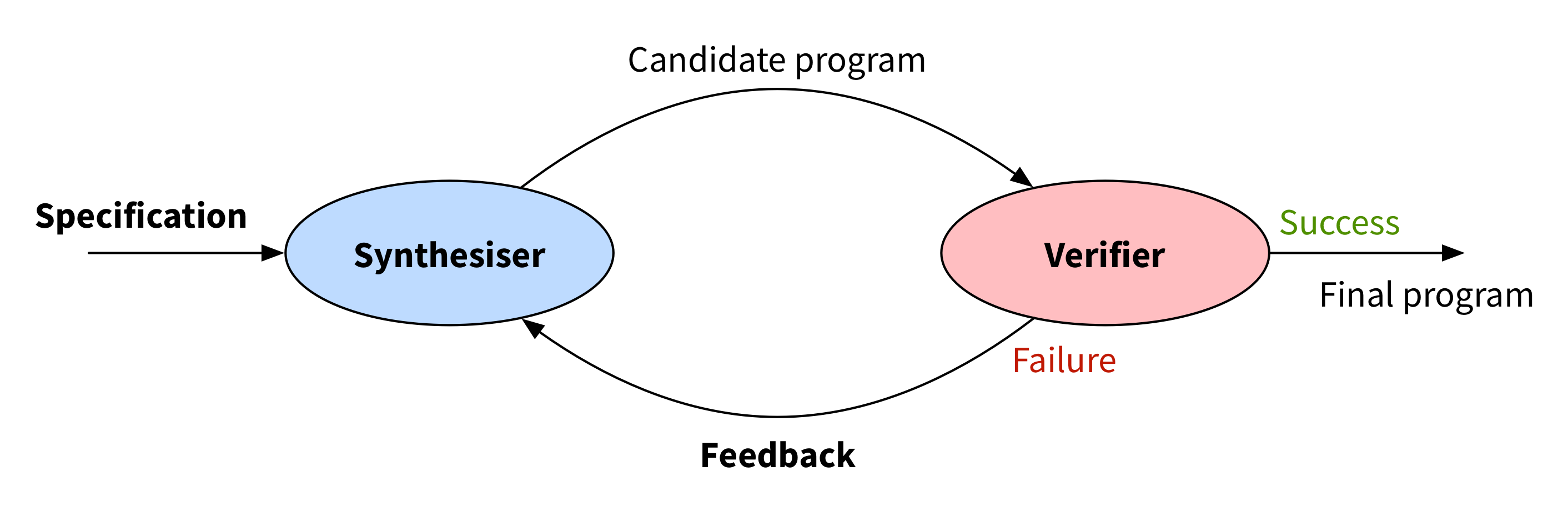
We start with some specification of the desired program. A synthesiser produces a candidate program that might satisfy the specification, and then a verifier decides whether that candidate really does satisfy the specification. If so, we’re done! If not, the verifier closes the loop by providing some sort of feedback to the synthesiser, which it will use to guide its search for new candidate programs.
It’s called “counterexample-guided” because the feedback is traditionally a counterexample – a new input on which the candidate program didn’t satisfy the specification. But I’m going to abuse this schematic a little and describe some techniques where the feedback isn’t really a counterexample.
There are a few holes we must fill to define a new CEGIS synthesis technique:
- how to specify the desired behaviour
- how to synthesise candidate programs
- how to verify a candidate program against the specification
- how to provide feedback for future candidates
So far we’ve said nothing about when or even if the CEGIS loop ever terminates. One of the strengths of many CEGIS techniques is their empirical tendency to require only very few trips around the loop, even though the space of programs is incredibly large.
I’m going to describe three different inductive program synthesis techniques that fit this CEGIS mold.
Oracle-guided synthesis
Jha et al’s oracle-guided synthesis assumes that you already have an implementation of the program you want to synthesise, which they call the oracle program. This implementation is the specification for oracle-guided synthesis. We treat the oracle as a black box we can execute on arbitrary inputs; we do not need to inspect the oracle’s implementation.
We also start with a collection of test cases, which are input-output pairs. Because we have an oracle, we can create test cases by just generating random inputs and asking the oracle for the correct answer for each.
Synthesis step
We provide oracle-guided synthesis with a library of components from which the synthesiser builds candidate programs. The synthesis step is going to arrange these components into a program in static single assignment form. In essence, it’s going to take all the components, and decide how to plug their inputs and outputs together to form a program. (This formulation disallows loops, so the programs we generate will always be loop-free.)
For example, here is a library of three components – two adds and a square root – and a possible way to connect them together:

The program those connections implement is in SSA form:
program(x, y):
    o1 = add(x, y)
    o2 = add(o1, y)
    o3 = sqrt(o1)
    return o3
Notice that we have two copies of the add component; the SSA form simply connects each component together, so if we want the final program to use two additions, we must supply at least two add components. Notice also that o2 is dead code since its output is unused. This is fine, and saves us from having to decide in advance exactly how many of each component the final program will use. Instead we only need to provide an upper bound, and the synthesiser can generate dead code for components it doesn’t want to use.
The synthesiser uses the test cases to constrain how the components can be linked together. It uses an SMT solver to decide which components to join together, such that the program is correct for all the test cases in the collection. If the SMT solver fails, then no program that uses only the given components can satisfy the test cases – the components are insufficient. Otherwise, it produces a program in SSA form that satisfies all the test cases (that is, P agrees with the oracle O on all the test inputs).
Verification step
If there is a solution, we pass the candidate program to the verify step. Remember that the candidate program satisfies all the test cases in the existing collection. The verify step is going to use an SMT solver to answer the question:
Does there exist another program P’, different from the candidate program P, that also satisfies all the test cases in the existing collection, but on some input z disagrees with P?
Let’s break this one down a bit. We have from the synthesiser a candidate program P that satisfies all the test cases. What we’re asking the verifier for now is a new test input z and a new program P’, so that for the input z, P and P’ produce different outputs. The new program P’ is also going to satisfy all the test cases.
Essentially, we’re asking if the program P is ambiguous – is there more than one program that could have satisfied all the test cases? If there is, we know we’re not done, since programs shouldn’t be ambiguous!
We’re not asking anything about the oracle program. In particular, it might be the case that P and P’ both produce wrong answers for input z; all that matters to the verifier is that they produce different answers.
For example, here’s how it works with two test cases and the same components we saw above:

Here the only test inputs we have are (0,0) and (1,0). The synthesiser gave us as a candidate P the program sqrt(x)+y, which satisfied both test cases since it agrees with the oracle on both. We asked the verifier to produce two things: a new program P’ and a new test input z. In this case, it was successful. It produced a new program x+y and a new test input (4,5). On this new test input, the candidate P and the new program P’ disagree: sqrt(4)+5 = 7, while 4+5 = 9. In this case, it turns out that both programs are wrong, since the oracle’s output for the new test case is sqrt(4+5) = 3. But the fact that P and P’ disagree is sufficient to send us back around the loop via the feedback step.
Feedback step
The feedback step is going to exploit the new test case z generated by the verifier. It asks the oracle O what the correct output is for input z, and adds the result to the set of test cases that the synthesiser will use in the next trip around the loop.
In the example, that next trip around the loop will be the last: the only way to use two adds and a square root to satisfy the (now three) test cases is the program sqrt(x+y). The question the verifier asks will therefore be unsatisfiable – it won’t be able to find a second program P’ – and so the loop will exit.
To be completely correct, we must also have some kind of validation oracle, which we consult after finishing the CEGIS loop. The problem is that the CEGIS loop is a race – will we find a unique program that satisfies the test cases before we find a test case that makes the components insufficient? If we find a unique program, we break the loop straight away. But we might have gotten lucky by not seeing a test case that proved that the components were insufficient. The validation oracle verifies that the synthesised program really does satisfy the specification on all inputs, not just a few test cases.
Starting with an existing program
Oracle-guided synthesis assumes you have an oracle, an existing implementation of the program you’re trying synthesise. We don’t actually need to inspect the implementation; we treat it as a black box that provides outputs when we supply inputs. But even this seems a little absurd: why synthesise a program we already have?
The authors use two domains to illustrate why their technique is useful. The first is the traditional suite of bit-vector benchmarks from Hacker’s Delight. Many synthesis papers use these benchmarks because they are examples of small, unintuitive programs. Instead of trying to come up with the most efficient bit-twiddling hack, programmers can write a simple, inefficient implementation of a bit-vector manipulation, and the synthesiser uses this implementation to produce an optimal program. The second domain is program de-obfuscation – taking an obfuscated program as the oracle, and synthesising a new, simpler program that matches its behaviour.
It’s worth noting that a follow-up paper to this one takes basically the same approach, but instead of requiring an oracle, requires a logical specification of the desired behaviour.
Stochastic superoptimisation
Schkufza et al’s stochastic superoptimisation is a completely different approach to program synthesis that I’ll attempt to beat into the CEGIS mold. Again, it assumes you have an existing implementation as the specification to compare against. This isn’t a problem for them, because as the name suggests, the problem they’re tackling is superoptimisation: finding the optimal instruction sequence for a given piece of code. Stochastic superoptimisation searches the space of programs to find a new program that matches the original’s behaviour but is faster or more efficient. It’s the search aspect that makes it a form of program synthesis.
Searching the space of programs
What’s the simplest way to search the space of programs? Suppose we start with a randomly generated program. To decide which program to try next, we could just randomly mutate one of the instructions in the program. Assuming the mutations satisfy some basic properties (for example, if the optimal program has an add instruction, the mutations must be able to generate an add instruction), this search will eventually find the optimal program. But this will probably take a very long time; there’s no guidance to decide if we’re on the right track, or “near” an answer.
Stochastic superoptimisation uses Markov-chain Monte Carlo (MCMC) sampling to search the space of programs in a more guided way. Essentially, stochastic superoptimisation defines a cost function that measures how “good” a candidate program is, and uses MCMC (in particular, the Metropolis algorithm) to sample programs that are highly weighted by that function. This bias means MCMC search is more likely to visit programs that are nearer to optimal. Although this is still a random search of a very large space, the bias means that empirically, stochastic superoptimisation often quickly discovers correct programs that are almost optimal.
Synthesis step
The synthesis step of stochastic superoptimisation finds the next candidate program P’ by drawing an MCMC sample based on the previous candidate program P. It proposes P’ by randomly applying one of a few mutations to P:
- changing the opcode of a randomly selected instruction
- changing a random operand of a randomly selected instruction
- inserting a new random instruction
- swapping two randomly selected instructions
- deleting an existing randomly selected instruction
The MCMC sampler uses the cost function, which measures how “close” to the target program P’ is and how fast P’ is, to decide whether to accept the candidate P’. A candidate is more likely to be accepted if it is close to the target or very fast. But even programs that are slow or distant from the target have some probability of being accepted, ensuring we explore novel programs (this is similar to the explore-exploit tradeoff in the multi-armed bandit problem).
If the candidate is accepted, we move on to the verification step. If not, we repeat this process until a candidate is accepted.
Verification step
Having accepted a candidate program P’, the verification step simply passes the candidate and target programs to a verifier to decide if they are equivalent. The paper has a few tricks to make this verification a little more forgiving of, for example, getting the correct result but in a different register.
The most important trick is that before executing the verifier, which could be slow, stochastic superoptimisation first uses the test cases from the cost function. If any of the test cases fail, we know the candidate can’t possibly be the correct program, and so there’s no need to call the verifier. Empirically, most bad candidates tend to fail fast on these test cases, and so this trick considerably improves the throughput of the MCMC search.
Feedback step
The feedback step of stochastic superoptimisation is implicit in the MCMC sampling. We compare new candidate programs P’ to the previously accepted candidate P to decide whether P’ is a program we should explore. If P’ is better than P (i.e. has a higher cost function, and so is either faster or closer to the target, or both) we are certain to explore it. Otherwise, there is still a probability of exploring P’; the probability depends on how much worse P’ is.
Enumerative search
The last synthesis technique I’m going to try to fit into the CEGIS mold is enumerative search. It’s a fairly obvious brute force approach with a neat trick, and despite its seeming naïveté, has been used to great effect, for example by Udupa et al in synthesising distributed systems protocols.
For a specification we’re going to use a finite set of test cases. Of course, since you can generate test cases given an implementation of the program, it’s fine to instead assume an existing implementation like we did with oracle-guided synthesis and stochastic superoptimisation. We also assume we have a grammar of the target language. For our purposes, we’ll use a simple grammar that has two operations add and sub, and two available variables x and y. The grammar defines expressions over these terms, so for example, add(x, sub(x, y)) is a program in this grammar. There’s no assignment statement, which will make our lives easier.
Synthesis step
The idea of enumerative search is to just brute force search all possible programs. We break programs up into depths based on the deepest path in their parse tree. For example, the program that just returns x has depth zero, while the program x+y has depth 1, and (x+y)+x has depth 2.
We synthesise candidate programs by starting at depth 0 and enumerating all programs at that depth. In our grammar, that means the first two candidates are just the two programs x and y. Once we’re done with a depth, we increment to the next depth and repeat the process. At depth 1, there are eight candidate programs, which all take the form operation(a, b):
Notice how the possible expressions for a and b are exactly the programs of depth 0. This is how we do the enumeration: at depth k, we explore all programs of the form operation(a, b), where a and b are any expression of depth at most k-1. This dynamic programming search is going to be exponential in the depth k: at depth 2, each hole can be filled with one of 8 depth-1 or 2 depth-0 expressions, and so we’ll have to explore 2×(8+2)² = 200 programs; at depth 3, we’ll have to explore 2×(200+8+2)² = 88,200 programs! We’ll rely on the feedback step to try to prune this search space.
Verification step
Because we specified the program in terms of test cases, the verification step is simply going to execute all the test cases and compare the output to the goal. If they match, we’re done.
Feedback step
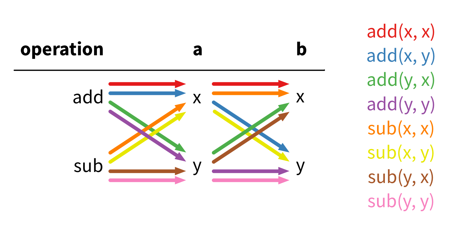
The test case output is also the key to the feedback step. The trick is that when trying to fill the holes in programs of depth k, we don’t need to consider every program of depth at most k-1. Instead, we need only consider those programs with distinct outputs. For example, there’s no point considering both sub(x, x) and sub(y, y) – they both have the same effect. This insight prunes the search space.
But how do we decide if two programs are distinct? That’s where the test cases come in. Because we defined the target program behaviour in terms of the test cases, it actually doesn’t matter if two programs are semantically different, but rather only whether they differ on the test cases. So to decide if a new program P is distinct from those we’ve seen so far, we simply compare its test case outputs to those from every other program. If it matches an existing program, there’s no point keeping P, and so we throw it away.
For example, if every test case has y = 0, then add(x, y) and sub(x, y) are equivalent, even though that’s clearly untrue in general. We get to prune a whole bunch of programs that are not semantically equivalent in general, but are equivalent for the set of behaviours we actually care about.
It turns out that this strategy works remarkably well for some problems. When synthesising cache coherence protocols, Udupa et al found that the pruning reduces the search space by a factor of nearly 100× at depth 10. Of course, how well it works on your problem will depend on both the set of behaviours you care about and the set of components you include in the grammar.
Conclusion
We’re not going to be synthesising entire applications from scratch any time soon, but that’s not really a viable goal anyway. In many cases, smaller programs are exactly what we’re after from synthesis: we can ask the programmer to bolt high-level pieces together, and fill in the minute details automatically. This is the idea of sketching, which prompted the original CEGIS work. It’s also an appeal to the 80-20 rule – programs spend most of their time in a few small areas of the code, and so synthesis on those small parts can still deliver significant efficiency improvements.
The promise of program synthesis is that programmers can stop telling computers how to do things, and focus instead on telling them what they want to do. Inductive program synthesis tackles this problem with fairly vague specifications and, although many of the algorithms seem intractable, in practice they work remarkably well. Chalk up another victory for the empiricists!
-
Sorry, Luis! We mock because we love. ↩
-
Some of my explanations are inspired by (my awesome adviser) Emina Torlak’s program synthesis course. All mistakes are my own! ↩