Deriving canonical correlation analysis
In which we explore CCA in detail
Canonical correlation analysis (CCA) is a statistical method for exploring the relationships between two sets of variables measured on the same sample. For example, suppose for a set of $n$ individuals we’ve measured $p$ variables related to health, such as blood pressure, cholestorol levels, body mass index, etc. Now suppose that for the same set of individuals we’ve also measured $q$ variables related to exercise, such as miles run per week, maximum bench press weight, etc. Given these two sets of measurements, we may want to explore how variables from the first set relate to those from the second set.
How might we go about this? One naive way would be to examine each possible pair of variables from the two sets of measurements. For example, we could make a scatter plot or perform linear regression on blood pressure vs. miles, blood pressurve vs. bench press, etc. However, this requires us to examine $p\cdot q$ pairs, which quickly becomes infeasible as $p$ or $q$ gets large. On the other hand, CCA summarizes these relationships into a much smaller number of statistics while preserving as much information as possible.
Here we’ll derive CCA mathematically as well as discuss some of its extensions.
Defining CCA
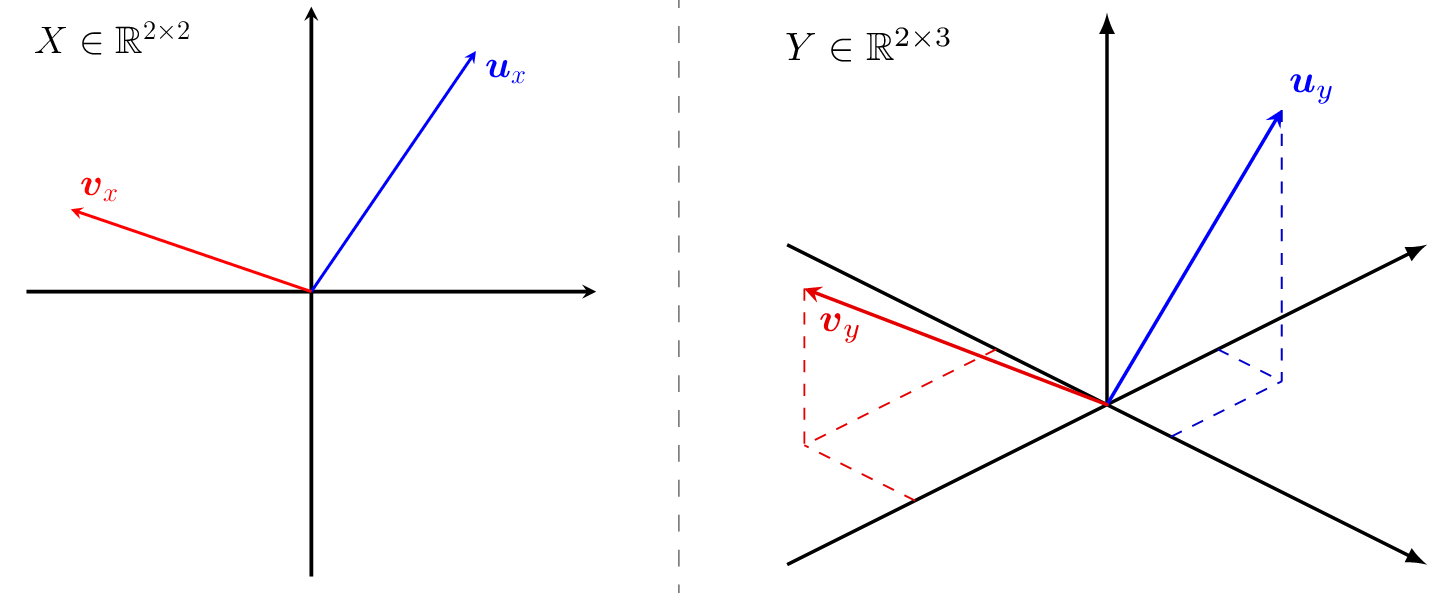
Suppose we have two paired datasets $X \in \mathbb{R}^{n \times p}$ and $Y \in \mathbb{R}^{n \times q}$. By paired we mean that the $i$’th rows of $X$ and $Y$ are drawn from the same sample. For simplicitly, we’ll assume that all the features of our data are zero-mean.
Now, let $\boldsymbol{w}_x \in \mathbb{R}^{p}$ and $\boldsymbol{w}_y \in \mathbb{R}^{p}$ denote linear transformations of $X$ and $Y$ respectively. The canonical variables $\boldsymbol{z}_x \in \mathbb{R}^n$ and $\boldsymbol{z}_y \in \mathbb{R}^n$ are then defined as
\[\boldsymbol{z}_x = X\boldsymbol{w}_x \quad \text{and} \quad z_y = Y\boldsymbol{w}_y.\]The objective of CCA is to learn the transformations $\boldsymbol{w}_x$ and $\boldsymbol{w}_y$ such that $\boldsymbol{z}_x$ and $\boldsymbol{z}_y$ are maximally correlated. In formal notation, the optimization problem we wish to solve is
Letting $\boldsymbol{\Sigma}_{xy}$ denote the cross-covariance matrix of $X$ and $Y$, we can write our objective as
\[\begin{aligned} \boldsymbol{w}_x^*, \boldsymbol{w}_y^* &= \underset{\boldsymbol{w}_x, \boldsymbol{w}_y}{\operatorname{argmax}} \text{corr}(\boldsymbol{z}_x, \boldsymbol{z}_y)\\ &= \underset{\boldsymbol{w}_x, \boldsymbol{w}_y}{\operatorname{argmax}} \text{corr}(X\boldsymbol{w}_x, Y\boldsymbol{w}_y) \\ &= \underset{\boldsymbol{w}_x, \boldsymbol{w}_y}{\operatorname{argmax}} \frac{\mathbb{E}[(X\boldsymbol{w}_x)^T(Y\boldsymbol{w}_y)]}{\sqrt{\mathbb{E}[(X\boldsymbol{w}_x)^{T}(X\boldsymbol{w}_x)]}\sqrt{\mathbb{E}[(Y\boldsymbol{w}_y)^T(Y\boldsymbol{w}_y)]}} \\ &= \underset{\boldsymbol{w}_x, \boldsymbol{w}_y}{\operatorname{argmax}} \frac{\boldsymbol{w}_x^T\mathbb{E}[X^TY]\boldsymbol{w}_y}{\sqrt{\boldsymbol{w}_x^T\mathbb{E}[X^{T}X]\boldsymbol{w}_x}\sqrt{\boldsymbol{w}_y^T\mathbb{E}[Y^TY]\boldsymbol{w}_y}} \\ &= \underset{\boldsymbol{w}_x, \boldsymbol{w}_y}{\operatorname{argmax}} \frac{\boldsymbol{w}_{x}^{T}\Sigma_{xy}\boldsymbol{w}_{y}}{\sqrt{\boldsymbol{w}_x^T\Sigma_{xx}\boldsymbol{w}_x}\sqrt{\boldsymbol{w}_y^T\Sigma_{yy}\boldsymbol{w}_y}} \end{aligned}\]Correlation is scale-invariant, so to make our lives easier we’ll constrain $||\boldsymbol{z}_x|| = ||\boldsymbol{z}_y|| = 1$. Our problem is thus to find $\boldsymbol{w}_x$ and $\boldsymbol{w}_y$ that satisfy
\[\begin{equation} \label{eq:cca_constrained} \max_{\boldsymbol{w}_x, \boldsymbol{w}_y} \boldsymbol{w}_{x}^{T}\boldsymbol{\Sigma}_{xy}\boldsymbol{w}_{y}\quad \text{s.t.}\ \ \boldsymbol{w}_x^T\boldsymbol{\Sigma}_{xx}\boldsymbol{w}_x = 1, \quad \boldsymbol{w}_y^T\boldsymbol{\Sigma}_{yy}\boldsymbol{w}_y = 1 \end{equation}\]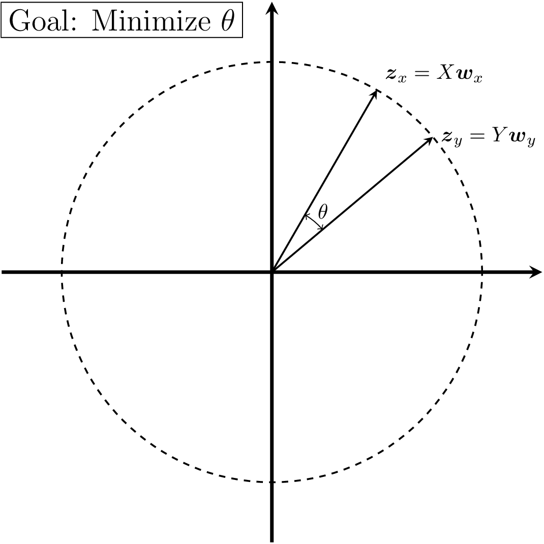
By adding these constraints, we can also obtain a more intuitive geometric interpretation of the CCA problem. Using our definitions of $\boldsymbol{z}_x$ and $\boldsymbol{z}_y$, we can rewrite (\ref{eq:cca_constrained}) as
\[\begin{equation} \max_{\boldsymbol{w}_x, \boldsymbol{w}_y} \mathbb{E}[\boldsymbol{z}_x^{T}\boldsymbol{z}_y]\quad \text{s.t.}\ \ ||\boldsymbol{z}_x|| = 1, \quad ||\boldsymbol{z}_y|| = 1, \end{equation}\]which, using the geometric interpretation of the dot product we can further rewrite as
\[\begin{equation} \max_{\boldsymbol{w}_x, \boldsymbol{w}_y} \cos{\theta} \quad \text{s.t.}\ \ ||\boldsymbol{z}_x|| = 1, \quad ||\boldsymbol{z}_y|| = 1, \end{equation}\]where $\theta$ is the angle between $\boldsymbol{z}_x$ and $\boldsymbol{z}_y$. As $\cos \theta$ is maximized at $\theta = 0$, we can interpret our problem as finding transformations $\boldsymbol{w}_x$ and $\boldsymbol{w}_y$ such that the resulting embeddings $\boldsymbol{z}_x$ and $\boldsymbol{z}_y$ are pointing in the same direction (Figure 2). Now let’s see how to actually find our transformations $\boldsymbol{w}_x$ and $\boldsymbol{w}_y$.
Solving the Problem
We’ll begin by rewriting our problem one last time to make our lives easier down the line. Define
\[\begin{aligned} \boldsymbol{\Omega} &= \boldsymbol{\Sigma}_{xx}^{-1/2}\boldsymbol{\Sigma}_{xy}\boldsymbol{\Sigma}^{-1/2}_{yy} \\ \boldsymbol{c} &= \boldsymbol{\Sigma}_{xx}^{1/2}{\boldsymbol{w}_x} \\ \boldsymbol{d} &= \boldsymbol{\Sigma}_{yy}^{1/2}{\boldsymbol{w}_y} \end{aligned}\]and then our problem becomes
\[\begin{equation} \label{eq:objective} \max_{\boldsymbol{w}_x, \boldsymbol{zw}_y} \boldsymbol{c}^{T}\boldsymbol{\Omega}\boldsymbol{d} \quad \text{s.t.}\ \ ||\boldsymbol{c}|| = 1, \quad ||\boldsymbol{d}|| = 1 \end{equation}\]We can then turn this constrained problem into an easier-to-solve unconstrainted problem using Lagrange multipliers, giving us
\[\mathcal{L} = \boldsymbol{c}^{T}\boldsymbol{\Omega}\boldsymbol{d} - \frac{\lambda_1}{2}(\boldsymbol{c}^{T}\boldsymbol{c} - 1) - \frac{\lambda_2}{2}(\boldsymbol{d}^{T}\boldsymbol{d} - 1).\]Now let’s take the derivatives of this equation with respect to $\boldsymbol{c}$ and $\boldsymbol{d}$. First, by applying matrix derivative rules we have
\[\begin{equation} \label{eq:partial_x} \frac{\partial \mathcal{L}}{\partial \boldsymbol{c}} = \boldsymbol{\Omega}\boldsymbol{d} -\lambda_1 \boldsymbol{c} = 0, \end{equation}\]Similarly, we can derive.
\[\begin{equation} \label{eq:partial_y} \frac{\partial \mathcal{L}}{\partial \boldsymbol{d}} = \boldsymbol{\Omega}^{T}\boldsymbol{c} - \lambda_2\boldsymbol{d} = 0. \end{equation}\]We’re left with two equations and four unknowns ($\lambda_1, \lambda_2, \boldsymbol{c},$ and $\boldsymbol{d}$). Now, let’s see if we can simplify things a bit. First, we’ll multiply Equation (\ref{eq:partial_x}) by $\boldsymbol{c}^T$. This gives us
\[\begin{aligned} 0 &= \boldsymbol{c}^T(\boldsymbol{\Omega}\boldsymbol{d} -\lambda_1 \boldsymbol{c}) \\ &= \boldsymbol{c}^T\boldsymbol{\Omega}\boldsymbol{d} - \lambda_1\boldsymbol{c}^T\boldsymbol{c}\\ &= \boldsymbol{c}^T\boldsymbol{\Omega}\boldsymbol{d} - \lambda_1\\ \end{aligned}\]Where we used our constraint $\boldsymbol{c}^T\boldsymbol{c} = 1$ to get the second equality. Similarly, by multiplying Equation (\ref{eq:partial_y}) by $\boldsymbol{d}^T$, we have
\[\begin{aligned} 0 &= \boldsymbol{d}^T(\boldsymbol{\Omega}^T\boldsymbol{c} - \lambda_2\boldsymbol{d})\\ &=\boldsymbol{d}^T\boldsymbol{\Omega}^T\boldsymbol{c} - \lambda_2\boldsymbol{d}^T\boldsymbol{d}\\ &= \boldsymbol{d}^T\boldsymbol{\Omega}^T\boldsymbol{c} - \lambda_2 \end{aligned}\]from which we can conclude $\lambda_1$ = $\lambda_2$. Define $\lambda = \lambda_1 = \lambda_2$. Plugging this into Equation (\ref{eq:partial_x}) we find
\[\begin{equation} \label{eq:singular_value} \boldsymbol{\Omega}\boldsymbol{d} = \lambda\boldsymbol{c}. \end{equation}\]That is, $\boldsymbol{d}$ and $\boldsymbol{c}$ must be right and left singular vectors of $\boldsymbol{\Omega}$ with a singular value of $\lambda$. Now, which specific singular vectors should we choose? Plugging Equation (\ref{eq:singular_value}) into our objective from Equation (\ref{eq:objective}), we get
\[\max_{\boldsymbol{w}_x, \boldsymbol{w}_y} \boldsymbol{c}^{T}\boldsymbol{\Omega}\boldsymbol{d} = \lambda \boldsymbol{c}^{T}\boldsymbol{c} = \lambda\]Thus implying that $\boldsymbol{d}$ and $\boldsymbol{c}$ must specifically be the right and left singular vectors of $\boldsymbol{\Omega}$ that correspond to the largest singular value $\lambda$.
Multiple Canonical Covariates
After solving the problem described previously, we’ll be able to project our data down to a single set of canonical variables. While this is a good start, by restricting ourselves to only a single set of variables, we’ll likely lose a good chunk of information. Thus, oftentimes we want to find a set of $r$ pairs of canonical variables with corresponding transformations $W_{x} \in \mathbb{R}^{p \times r}$ and $W_{y} \in \mathbb{R}^{q \times r}$, where the $i$th column of these matrices represents a mapping to the $i$th canonical covariate. To ensure that each pair of canonical variables is capturing different phenomena, we’ll restrict them to be uncorrelated/orthogonal to each other, i.e:
\[(\boldsymbol{z}_{x}^{i})^T\boldsymbol{z}_x^{j} = 0, \quad (\boldsymbol{z}_{y}^{i})^{T}\boldsymbol{z}_y^{(j)} = 0 \quad \forall j \neq i : i,\ j \in \{1, \ldots, r\}\]where $(\boldsymbol{z}_{x}^{i}, \boldsymbol{z}_{y}^{i})$ is the $i$th pair of canonical variables. As it turns out, we satisfy this additional constraint without any additional work. To see this, we can define $\boldsymbol{w}_{x}^{i}$ and $\boldsymbol{w}_{y}^{i}$ such that
\[\boldsymbol{z}_x^i = X\boldsymbol{w}_x^i \quad \text{and} \quad \boldsymbol{z}_y^i = Y\boldsymbol{w}_y^i.\]and similarly $\boldsymbol{c}^i$ and $\boldsymbol{d}^i$ such that
\[\begin{aligned} \boldsymbol{c}^i &= \boldsymbol{\Sigma}_{xx}^{1/2}{\boldsymbol{w}_x^i} \\ \boldsymbol{d}^i &= \boldsymbol{\Sigma}_{yy}^{1/2}{\boldsymbol{w}_y^i} \end{aligned}\]Using our previous analysis, we can conclude that any optimal $(\boldsymbol{z}_{x}^{i}, \boldsymbol{z}_{y}^{i})$ must correspond to a $\boldsymbol{c}^i$ and $\boldsymbol{d}^i$ that are singular vectors with the $i$th largest singular values of the matrix $\boldsymbol{\Omega}$ defined previously. As it turns out, for a given matrix any two right or left singular vectors are orthogonal. That is, we must have
\[(\boldsymbol{c}^{i})^T\boldsymbol{c}^j = 0, \quad (\boldsymbol{d}^{i})^T\boldsymbol{d}^j = 0.\]With a little algebra, we can show that
\[(\boldsymbol{c}^{i})^T\boldsymbol{c}^j = 0 \iff (\boldsymbol{z}_x^{i})^T\boldsymbol{z}_x^j = 0, \quad (\boldsymbol{d}^{i})^T\boldsymbol{d}^j = 0 \iff (\boldsymbol{z}_y^{i})^T\boldsymbol{z}_y^j = 0,\]thus guaranteeing that we satisfy the orthogonality constraint automatically.
Finally, we’ll discuss briefly the number of canonical variables $r$. Since the solutions to our optimization problem must be singular vectors of $\boldsymbol{\Omega}$, $r$ cannot be greater than the number of singular vectors of $\boldsymbol{\Omega}$.
How many singular vectors does $\Omega$ have? Recall that we defined $\boldsymbol{\Omega}$ as
\[\boldsymbol{\Omega} = \boldsymbol{\Sigma}_{xx}^{-1/2}\boldsymbol{\Sigma}_{xy}\boldsymbol{\Sigma}^{-1/2}_{yy}\]Assuming that our data matrices $X \in \mathbb{R}^{n \times p}$ and $Y\in \mathbb{R}^{n \times q}$ do not have any redundant features, the cross-covariance matrix $\boldsymbol{\Sigma}_{xy}$ has rank $\min(p, q)$. Moreover, the matrices $\boldsymbol{\Sigma}_{xx}^{-1/2}$ and $\boldsymbol{\Sigma}_{yy}^{-1/2}$ are full-rank with rank $p$ and $q$ respectively. Multiplying a matrix by a full-rank matrix preserves rank, so we can conclude that $\text{rank}(\boldsymbol{\Omega}) = \min(p, q)$. Since the number of singular vectors of a matrix is equal to its rank, we must choose $r \leq \min(p, q)$.