Hyperband: A Novel Bandit-Based Approach to Hyperparameter Optimization
Kevin Jamieson on joint work with Lisha Li, Giulia DeSalvo, Afshin Rostamizadeh, and Ameet Talwalkar (https://arxiv.org/abs/1603.06560)
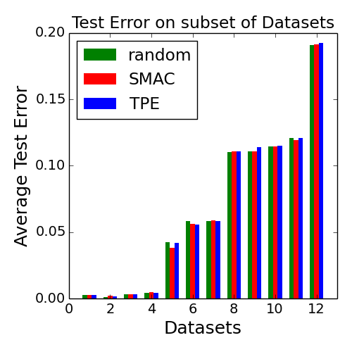
The hyperparamter optimization literature in recent years has been dominated by hyperparameter selection algorithms (e.g. Bayesian Optimization) that attempt to improve upon grid/random search. However, recent evidence on a benchmark of over a hundred hyperparameter optimization datasets suggests that such enthusiasm may call for increased scrutiny. Rank plots aggregate statistics across datasets for different methods as a function of time: first place gets one point, second place two points, and so forth. The plot, reproduced from that work, is the average score across 117 datasets collected by Feurer et. al. 2015 (lower is better).
Random search appears to be soundly beat by the state-of-the-art Bayesian optimization methods of SMAC (Hutter et al 2011) and TPE (Bergstra et al 2011), which is presumably expected. However, if we look at 12 randomly sampled datasets from these 117 (the story is the same for any subset) and plot their test error after one hour, we observe that none of SMAC, TPE, or random clearly outperforms any other. What we conclude from these two plots is that while the Bayesian Methods perhaps consistently outperform random sampling, they do so only by a negligible amount. To quantify this idea, we compare to random run at twice the speed which beats the two Bayesian Optimization methods, i.e., running random search for twice as long yields superior results (Spearmint (Snoek et al 2012) omitted due to complications with conditional hyperparmeters).
A critical reader may ask if this is a fair comparison since if the number of evaluations in an hour is smaller than the dimensionality of the search space, there is no hope to beat random by substantial amount. However, in this highly structured search space, the intrinsic dimensionality of the hyperparameter space is about 15. Random sampling on more than half the datasets gets at least 200 evaluations, one quarter of datasets get 400 evaluations. At least some Bayesian Optimization advocates say this number of evaluations is more than enough. Thus, while we by no means believe that these 117 datasets represent all possible datasets, it is a valid and fair comparison.
This observation led my coauthors and I to pursue an alternative approach. In particular, we employ recent advances in pure-exploration algorithms for multi-armed bandits to exploit the iterative algorithms of machine learning and embarrassing parallelism of hyperparmeter optimization. In contrast to treating the problem as a configuration selection problem, we pose the problem as a configuration evaluation problem and select configurations randomly. By computing more efficiently, we look at more hyperparameter configurations - more than making up for the ineffectiveness of random search used for selection - and outperform state-of-the-art Bayesian Optimization procedures.
Our procedure, HYPERBAND is parameter-free and has strong theoretical guarantees for correctness and sample complexity. The approach relies on an early-stopping strategy for iterative algorithms of machine learning algorithms. The rate of convergence does not need to be known in advance and, in fact, our algorithm adapts to it so that if you replace your iterative algorithm with one that converges faster, the overall hyperparameter selection process is that much faster. This post is intended to give an introduction to the approach and present some promising empirical results.
Hyperband Algorithm
The underlying principle of the procedure exploits the intuition that if a hyperparameter configuration is destined to be the best after a large number of iterations, it is more likely than not to perform in the top half of configurations after a small number of iterations. That is, even if performance after a small number of iterations is very unrepresentative of the configurations absolute performance, its relative performance compared with many alternatives trained with the same number of iterations is roughly maintained. There are obvious counter-examples; for instance if learning-rate/step-size is a hyperparameter, smaller values will likely appear to perform worse for a small number of iterations but may outperform the pack after a large number of iterations. To account for this, we hedge and loop over varying degrees of the aggressiveness balancing breadth versus depth based search. Remarkably, this hedging has negligible effect on both theory (a log factor) and practice.
HYPERBAND requires 1) the ability to sample a hyperparameter configuration (get_random_hyperparameter_configuration()), and 2) the ability to train a particular hyperparameter configuration until it has reached a given number of iterations (perhaps resuming from a previous checkpoint) and get back the loss on a validation set (run_then_return_val_loss(num_iters=r,hyperparameters=t)). Uniform random sampling is the obvious choice as it is typically trivial to implement over categorical, continuous, and highly structured spaces, but our procedure is indifferent to the sampling distribution: the better the distribution you define, the better the procedure performs. Nearly every iterative algorithm (e.g. gradient methods) will expose the ability to specify a maximum iteration making the two requirements of our procedure generally applicable. Consider the following python code snippet, the entirety of the codebase of Hyperband.
# you need to write the following hooks for your custom problem
from problem import get_random_hyperparameter_configuration,run_then_return_val_loss

max_iter = 81  # maximum iterations/epochs per configuration
eta = 3 # defines downsampling rate (default=3)
logeta = lambda x: log(x)/log(eta)
s_max = int(logeta(max_iter))  # number of unique executions of Successive Halving (minus one)
B = (s_max+1)*max_iter  # total number of iterations (without reuse) per execution of Succesive Halving (n,r)

#### Begin Finite Horizon Hyperband outlerloop. Repeat indefinetely.
for s in reversed(range(s_max+1)):
    n = int(ceil(int(B/max_iter/(s+1))*eta**s)) # initial number of configurations
    r = max_iter*eta**(-s) # initial number of iterations to run configurations for

    #### Begin Finite Horizon Successive Halving with (n,r)
    T = [ get_random_hyperparameter_configuration() for i in range(n) ]
    for i in range(s+1):
        # Run each of the n_i configs for r_i iterations and keep best n_i/eta
        n_i = n*eta**(-i)
        r_i = r*eta**(i)
        val_losses = [ run_then_return_val_loss(num_iters=r_i,hyperparameters=t) for t in T ]
        T = [ T[i] for i in argsort(val_losses)[0:int( n_i/eta )] ]
    #### End Finite Horizon Successive Halving with (n,r)
For s=s_max, in the time a naive computation would consider logeta(max_iter) configurations, Hyperband considers max_iter configurations.
The outerloop describes the hedge strategy alluded to above and the innerloop describes the early-stopping procedure that considers multiple configurations in parallel and terminates poor performing configurations leaving more resources for more promising configurations.
The term iteration is meant to indicate a single unit of computation (e.g. an iteration could be .5 epochs over the dataset) and without loss of generality min_iter=1. Consequently, the length of an iteration should be chosen to be the minimum amount of computation where different hyperparameter configurations start to separate (or where it is clear that some settings diverge). Typically an iteration is defined as a constant fraction of the dataset size.
We suggest that max_iter be set to the number of iterations you would use if your boss gave you a hyperparameter configuration and asked for a model back. The parameter eta can be kept at the default (the theory suggests setting eta=e=2.7183...) but can also be changed for practical purposes as it controls the value of B: the total number of iterations taken for a particular run of Successive Halving (n,s).
The sweeping of s=0,...,s_max trades off breadth versus depth.
The following table describes the number of configurations n_i and the number of iterations they are run for r_i within each round of the Successive Halving innerloop for a particular value of (n,s).
max_iter = 81        s=4             s=3             s=2             s=1             s=0
eta = 3              n_i   r_i       n_i   r_i       n_i   r_i       n_i   r_i       n_i   r_i
B = 5*max_iter       ---------       ---------       ---------       ---------       ---------
                      81    1         27    3         9     9         6     27        5     81
                      27    3         9     9         3     27        2     81
                      9     9         3     27        1     81
                      3     27        1     81
                      1     81
Each inner loop indexed by s is designed to take B total iterations.
Intuitively, this means each value of s takes about the same amount of time on average.
For large values of s the algorithm considers many configurations (max_iter at the most) but discards hyperparameters based on just a very small number of iterations which may be undesirable for hyperparameters like the learning_rate. For small values of s the algorithm will not throw out hyperparameters until after many iterations have been performed but fewer configurations are considered (logeta(max_iter) at the least). The outerloop hedges over all possibilities.
Experimental Results
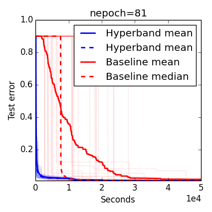
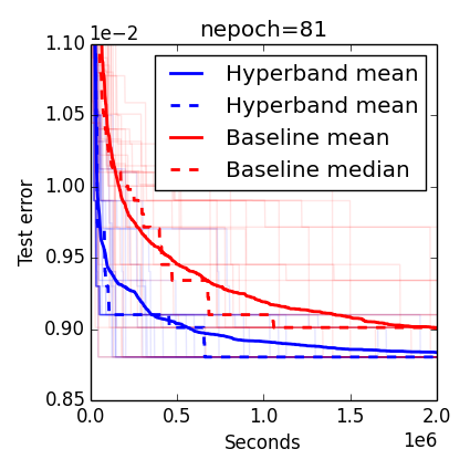
Our paper describes a number of extensions, theoretical guarantees, and fascinating implications for stochastic infinite-armed bandit problems. Here, we present some empirical evidence that it actually works.LeNet, SGD on MNIST (warmup)
We study the LeNet Convolutional Neural Network solver that implements mini-batch SGD on the MNIST dataset available at http://deeplearning.net/tutorial/lenet.html. The solver requires no modification as we only specify the hyperparameter setting and the number of iterations to run for. Each hyperparameter setting is drawn randomly according to the table.
| Hyperparameter | Scale | Min | Max |
| Learning Rate | log | 1e-3 | 1e-1 |
| Batch size | log | 1e1 | 1e3 |
| Layer 2 Num Kernels (k2) | linear | 10 | 60 |
| Layer 1 Num Kernels (k1) | linear | 5 | k2 |
The baseline method simply runs for a maximum number of epochs max_iter. These experiments used the exact configuration used in the code above. In all plots that follow, the algorithm only uses validation error to make keep-or-kill-decisions or what hyperparameters to recommend.
We report test error of the methods' resulting recommendations. Experimental results are reported in seconds and aggregated statistics for curves are the result of about 70 repeated trials on Amazon Web Services c4.large instances.
Comparison (low accuracy)
Comparison (high accuracy)
S-comparison
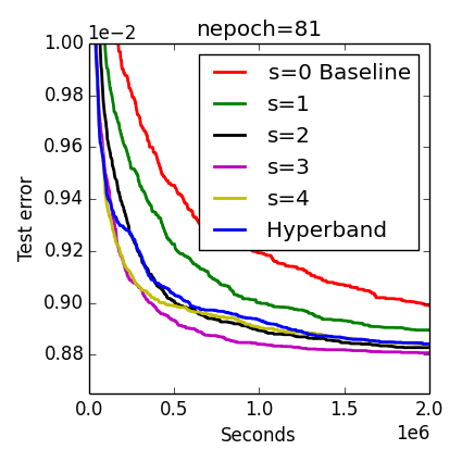
As discussed above, Hyperband sweeps over different values of s since one value will work best for identifying good parameters using the least effort possible, but this best value is not known a priori.
While the non-adaptive round-robin sweep over different values of s appears naive, one observes in the last plot that Hyperband nearly keeps up with the single best value of s=3 that is neither one of the extremes of s=4 or s=0 (baseline).
Cudaconvnet on Cifar-10, SVHN, MRBI (deep learning)
We consider three image classification datasets: CIFAR-10, Street View House Numbers (SVHN), and rotated MNIST with background images (MRBI). CIFAR-10 and SVHN contain 32 x 32 RGB images while MRBI contains 28 x 28 grayscale images. Each dataset is split into a training, validation, and test set: (1) CIFAR-10 has 40,000, 10,000, and 10,000 instances; (2) SVHN has close to 600,000, 6,000, and 26,000 instances; and (3) MRBI has 10,000 , 2,000, and 50,000 instances for training, validation, and test respectively. For all datasets, the only preprocessing performed on the raw images was demeaning.
| Hyperparameter | Scale | Min | Max |
| Initial Learning Rate | log | 5e-5 | 5 |
| Learning Rate Reductions | integer | 0 | 3 |
| Conv1 l2 penalty | log | 5e-5 | 5 |
| Conv2 l2 penalty | log | 5e-5 | 5 |
| Conv3 l2 penalty | log | 5e-5 | 5 |
| FC4 l2 penalty | log | 5e-5 | 5 |
| Response normalization scale | log | 5e-6 | 5 |
| Response normalization power | linear | 1e-2 | 3 |
We ran HYPERBAND with an "iteration" corresponding to 10,000 examples of the dataset (trained with minibatch SGD of minibatches of size 100). We set max_iter=300 for CIFAR-10 and MRBI (note, for CIFAR this corresponds to 75 epochs over the training set), while a maximum iteration of max_iter=600 was used for SVHN
due to its larger training set. We specified eta=4 for all experiments; this limited the number
of iterations of SUCCESSIVEHALVING to at most 5, thus allowing each iteration of HYPERBAND
to complete within reasonable times.
The same cuda-convnet architecture of Snoek et al 2015 and Domhan et al 2015 was used with a slightly different hyperparameter search space (i.e. direct comparison between these works is apples to oranges). The following plots are curves of the mean of 10 trials (not the min of 10 trials, see forthcoming paper) SMAC (Hutter et al 2011), SMAC-early-(stopping) (Donham et al 2015), TPE (Bergstra et al 2011), and Spearmint (Snoek et al 2012) are three state-of-the-art Bayesian Optimization solvers. Note that SMAC-early attempts to fit convergence behavior of iterative algorithms and performs early stopping like Hyperband. However, instead of trying to fit curves, Hyperband applies an algorithm that adapts to the unknown convergence behavior automatically.
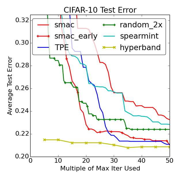
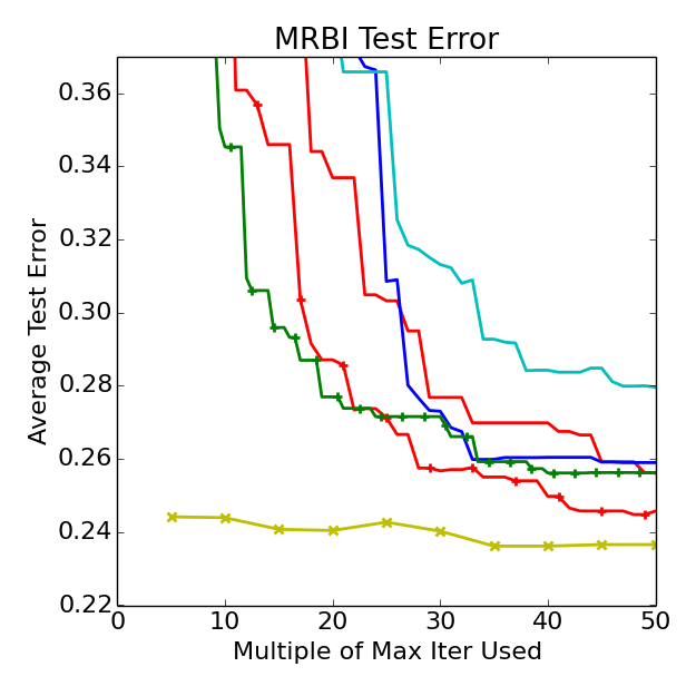
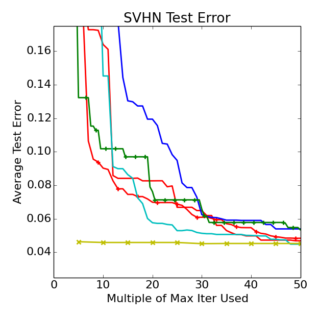
While random and the Bayesian Optimization algorithms output their first recommendation after max_iter iterations, Hyperband does not output anything until about max_iter(logeta(max_iter)+1) iterations, but when it does Hyperband has already considered 256 configurations whereas at this point the other methods have considered just (logeta(max_iter)+1)=5 configurations. This drastic difference in the number of considered configurations may explain Hyperband's considerable early lead.
Background and Related Work
Hyperparameter tuning first came to my attention when Ameet Talwalkar approached me about some empirical results in a preprint he and his coauthors were preparing for a larger systems paper (Sparks et al 2015). That work showed on 5 SVM hyperparameter selection benchmarks that random search was competitive with state-of-the-art Bayesian Optimization methods. Aiming to exploit this observation, they proposed an early-stopping heuristic that resembles the innerloop of Hyperband that sped up hyperparameter selection on their benchmarks by more than an order of magnitude. Recognizing the similarities of their heuristic with the Successive Halving algorithm of Karnin et al 2013 which was designed for the pure exploration stochastic multi-armed bandit (MAB) problem, Ameet and I defined the pure exploration non-stochastic MAB problem and proposed using the same algorithm. In Jamieson and Talwalkar 2016 we provided a novel analysis of Successive Halving for this non-stochastic setting and showed promising empirical results for hyperparameter optimization using iterative machine learning algorithms.
One drawback of this initial work with Ameet is that it considered only a fixed, finite set of hyperparameter configurations and provided no guidance on how to grow the number of configurations over time. This was taken care of by using a sequential cover over larger and larger sets of configurations as time increased (analogous to the outerloop of Hyperband) allowing us to define the pure exploration non-stochastic infinite-armed bandit problem (Li, Jamieson, Desalvo, Rostamizadeh, Talkwalkar, 2016). Because the non-stochastic problem is a generalization of the stochastic problem, our algorithm applied to the stochastic setting and turned out to be the first algorithm for that problem that adapted to unknown problem-dependent parameters and moreover, we proved that our algorithm is within log factors of the best known lower bounds (Carpentier et al 2015). However, after consulting with practitioners we kept hearing that they desired a max_iter - the maximum number of iterations a configuration would ever be trained for - resulting in the "finite horizon" version of Hyperband presented above. It shares many of the same theoretical properties as its original "infinite horizon" counterpart but allows it to be applied more generally. For instance, "iterations" could be replaced by downsampling the size of the dataset or number of features, quantities that often have a finite maxima.
Also in this paper we (and by we I mean almost exclusively Lisha Li at UCLA) performed all the experiments and comparisons to Bayesian Optimization found in this post.
Sparks et al 2015 and our follow-up works were certainly not the first to consider early-stopping for hyperparameter optimization. Indeed, such approaches have been given theoretical (Gyorgy et al 2011, Agarwal et al 2011) and practical (Swersky et al 2014, Domhan et al 2015) attention. However, all of these approaches either explicitly assume a form for the convergence behavior of the iterative method (e.g. c/sqrt(t) for some c) or attempt to identify a convergence behavior among a particular class as a function of hyperparameter configuration while performing hyperparameter optimization. These approaches are undesirable as convergence behavior can change from dataset to dataset and the success of the approach is linked to the expertise of the practitioner selecting possible convergence behaviors. In contrast, our method adapts to unknown convergence behavior automatically so that if you replace your gradient method with a faster Newton method, for instance, the Hyperband algorithm does not change, it just finds hyperparameters that much faster.
Extensions
The appeal of the Hyperband algorithm is its simplicity, theoretical guarantees of correctness, and its ability to adapt to unknown convergence behavior of iterative algorithms. It is also ripe for plugging in the successes of related work. For instance, it is natural to sample hyperparameters uniformly at random in get_random_hyperparameter_configuration(), but one could also consider a distribution that evolves over time as more evaluations are collected as is explored in Loshchilov et al 2016, effectively combining the adaptive selection ideas of Bayesian Optimization and adaptive computation of Hyperband.
Indeed, the meta-learning ideas developed in Feurer et al 2015 to build better priors for Bayesian Optimization could just as well be used as prior distributions to sample from in palce of uniform random sampling. Also, while we downsample iterations, numbers of features or dataset size could just as easily be downsampled, a particularly attractive option when training time is superlinear in these quantities.
Alternatively, the outerloop of Hyperband simply loops around the different values of s but conceivably one could treat the search for the best value of s as some sort of meta-multi-armed bandit game where each value of s is a different meta-arm, epsilon-greedy methods may perform well here. Finally, we remark that hyperparameters appear far beyond just machine learning applications and that Hyperband may be very useful in tuning coupled backend real-time systems that are typically tuned in isolation (e.g. number of worker threads, prefetch size, database configuration). We believe the flexibility of the algorithm and the weak assumptions necessary for theoretical guarantees make it a useful generic tool for many domains.
References
- Feurer, M., Klein, A., Eggensperger, K., Springenberg, J., Blum, M., & Hutter, F. (2015). Efficient and Robust Automated Machine Learning. In Advances in Neural Information Processing Systems (pp. 2944-2952).
- Snoek, Jasper, et al. "Scalable Bayesian Optimization Using Deep Neural Networks." Proceedings of the 32nd International Conference on Machine Learning (ICML-15). 2015.
- Hutter, F., Hoos, H., and Leyton-Brown., K. Sequential model-based optimization for general algorithm configuration. In Proc. of LION-5, 2011.
- Bergstra, James S., et al. "Algorithms for hyper-parameter optimization." Advances in Neural Information Processing Systems. 2011.
- Snoek, J., Larochelle, H., and Adams, R. Practical bayesian optimization of machine learning algorithms. In NIPS, 2012.
- E. Sparks, A. Talwalkar, D. Haas, M. J. Franklin, M. I. Jordan, T. Kraska. "Automating Model Search for Large Scale Machine Learning," In Symposium on Cloud Computing, 2015.
- Karnin, Zohar, Tomer Koren, and Oren Somekh. "Almost optimal exploration in multi-armed bandits." Proceedings of the 30th International Conference on Machine Learning (ICML-13). 2013.
- K. Jamieson and A. Talwalkar. "Non-stochastic Best Arm Identification and Hyperparameter Optimization," in the Proceedings of the 19th International Conference on Artificial Intelligence and Statistics, pp. 240-248, 2016.
- Lisha Li, Kevin Jamieson, Giulia DeSalvo, Afshin Rostamizadeh, and Ameet Talwalkar. "Efficient Hyperparameter Optimization and Infinitely Many Armed Bandits." arXiv preprint arXiv:1603.06560 (2016).
- Carpentier, Alexandra, and Michal Valko. "Simple regret for infinitely many armed bandits." 32th International Conference on Machine Learning. 2015.
- Gyorgy, A. and Kocsis, L. Efficient multi-start strategies for local search algorithms. JAIR, 41, 2011.
- Agarwal, A., Duchi, J., Bartlett, P. L., and Levrard, C. Oracle inequalities for computationally budgeted model selection. In COLT, 2011.
- Swersky, K., Snoek, J., and Adams, R. P. Freeze-thaw bayesian optimization. arXiv preprint arXiv:1406.3896, 2014.
- Domhan, T., Springenberg, J. T., and Hutter, F. Speeding up automatic hyperparameter optimization of deep neural networks by extrapolation of learning curves. In IJCAI, 2015.
- Ilya Loshchilov, and Frank Hutter. "CMA-ES for Hyperparameter Optimization of Deep Neural Networks." arXiv preprint arXiv:1604.07269 (2016).