suppressPackageStartupMessages({
  library(tidyverse)
  library(gganimate)
  library(gifski)
})Statistical modeling
Tutorial
Packages used
Random seed
Fix the random seed for reproducibility.
set.seed(1)The actual seed value doesn’t really matter here. We fix it so that we can refer to particular samples.
Uniform distribution
1M data points, uniformly distributed between 0 and 10.
uni <- tibble(Value=runif(1000000, 0, 10))This creates a tibble with a single column Value.
Mean and standard deviation
mean(uni$Value)[1] 4.999223sd(uni$Value)[1] 2.886293Recall that uni$Value indexes the column Value in tibble (data frame) uni.
Density plot
Plot the density of all values in column Value in the tibble (data frame) uni.
ggplot(uni, aes(x=Value)) + geom_density() + theme_bw()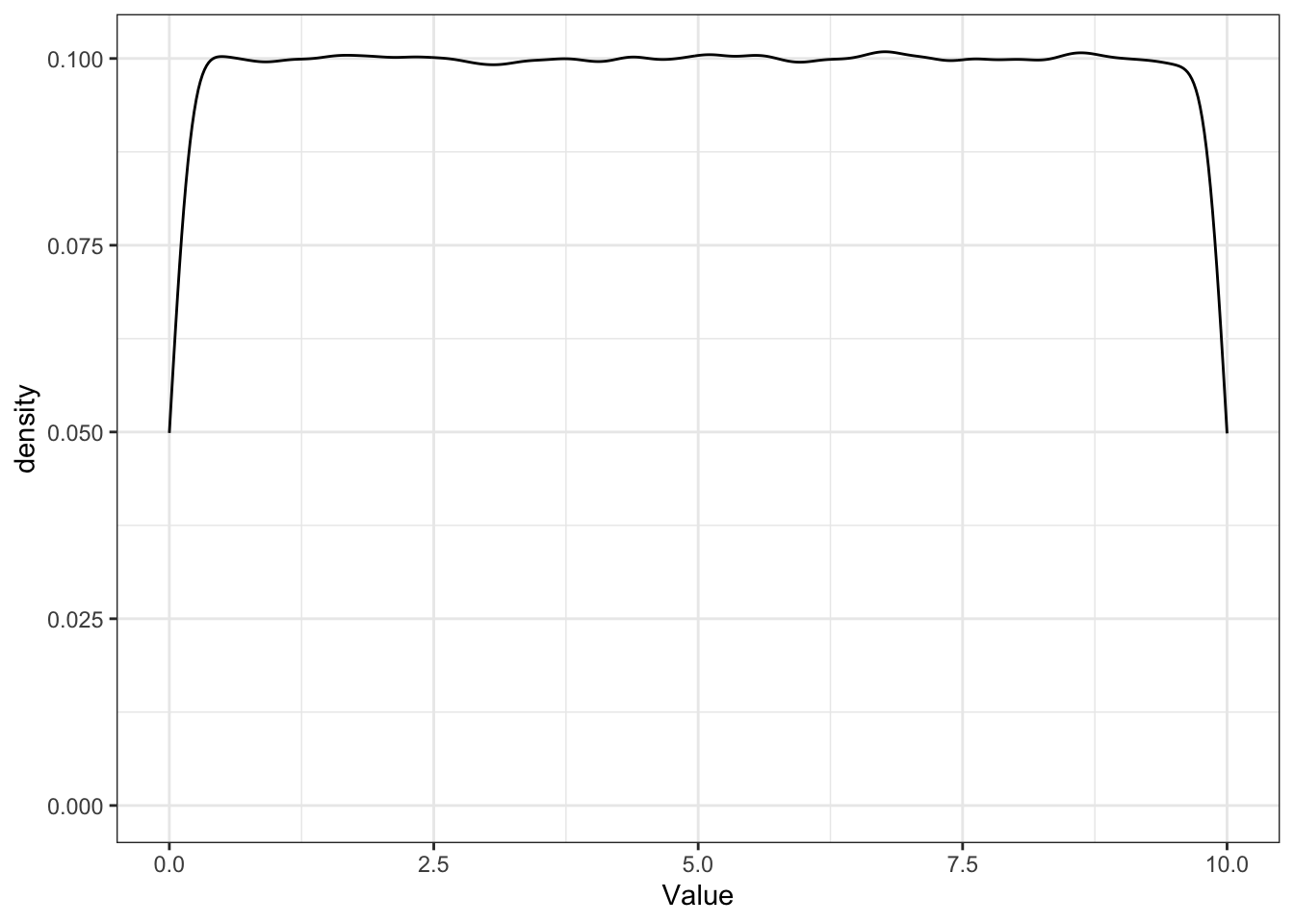
Drawing samples
Create a total of 10 samples and sample 10 values from the population for each.
S <- 10
N <- 100

l <- replicate(S, sample(uni$Value, N, replace=F), simplify=F)

# Name each entry in the list
names(l) <- seq(1, S)

# Create a tibble from the list
samples.wide <- as_tibble(l)

# What does this tibble look like?
samples.wide
# A tibble: 100 × 10
`1` `2` `3` `4` `5` `6` `7` `8` `9` `10`
<dbl> <dbl> <dbl> <dbl> <dbl> <dbl> <dbl> <dbl> <dbl> <dbl>
1 6.97 7.79 4.33 5.11 3.16 6.77 1.10 5.07 7.49 7.59
2 4.91 2.53 7.34 5.95 7.37 5.78 2.56 5.12 8.60 5.69
3 6.99 1.32 5.11 3.65 5.25 5.15 2.90 4.60 5.91 0.723
4 9.68 0.565 8.65 7.96 5.87 2.38 8.94 0.468 7.78 9.67
5 6.54 6.60 5.08 4.11 1.17 3.09 9.25 0.426 4.08 7.65
6 8.50 3.94 7.59 9.67 3.77 0.135 0.558 3.26 4.92 4.93
7 5.35 5.86 7.13 1.92 7.62 0.835 9.97 4.64 8.36 1.61
8 6.36 9.30 0.517 7.86 3.92 1.67 4.05 9.36 9.74 3.30
9 8.80 5.68 0.863 3.13 8.90 2.80 5.63 5.08 9.75 7.03
10 8.80 5.80 6.92 4.78 2.48 7.93 4.50 1.10 2.60 6.72
# ℹ 90 more rows# samples.long <- ...Creates a tibble with S columns – each a sample from the population.
The call to
samplesamplesNvalues fromuni$Valuewithout replacement.replicaterepeats the call tosampleStimes and returns a list of samples. We simply enumerate the samples from1toSand use the sample id as column name.
Wide to long data
There many ways of creating a tibble in long format.
You can use your R magic to convert from wide to long, or create a tibble in long format directly (e.g., bind_rows).
Plot the population and all samples.
The population from which we sample is plotted in black. The samples from this population are color-coded.
ggplot() + geom_density(data=samples.long, aes(x=Value, color=Sample, color=Sample)) +
           geom_density(data=uni, aes(x=Value), color="black") +
           theme_minimal()
Warning: Duplicated aesthetics after name standardisation: colour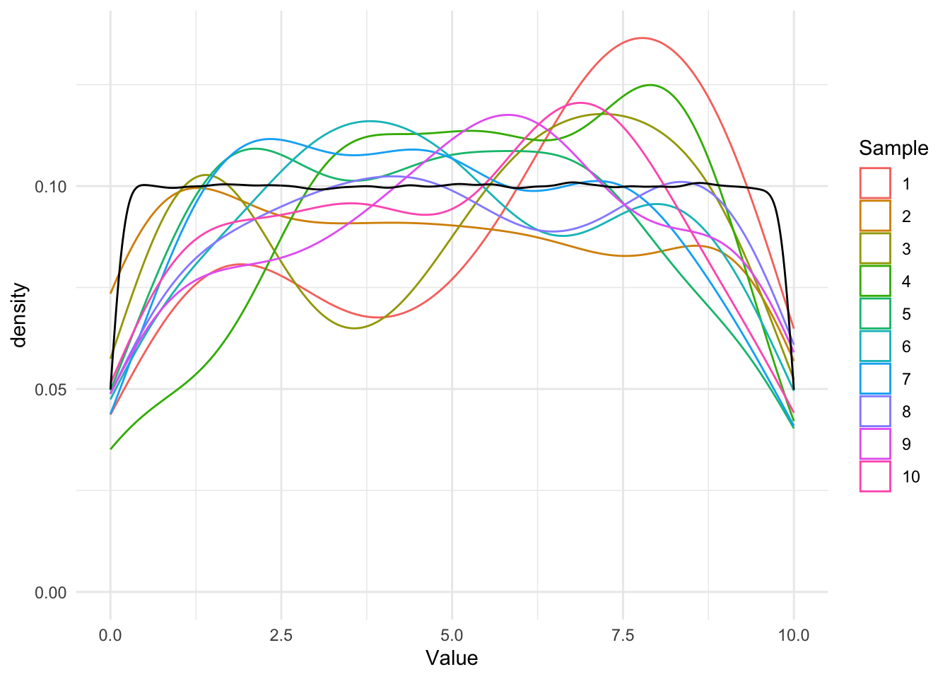
Notes
Each geom_density uses a different tibble (data frame).
Setting
colororfillwithin the aestheticsaesleads to- grouping of values by labels and
- each density plot having a different line color. This example uses a default color palette, which can be changed. (Note: If
samplewas a numeric column, a color gradient would be used in stead of distinct colors.)
Setting
coloroutside the aestheticsaesleads to a single line color for the entire plot.When breaking lines, make sure to put the
+at the end of the line, not on the new line.
Simulations
Animated plot of samples
Let’s plot the population and each sample again, but with an animation.
p <- ggplot() + geom_density(data=samples.long, aes(x=Value, color=Sample, fill=Sample)) +
           geom_density(data=uni, aes(x=Value), color="black") +
           theme_minimal() +
           labs(title = "Sample: {current_frame}") +
           transition_manual(Sample)
animate(p, fps=20)
`nframes` and `fps` adjusted to match transition
Galton board
Another example for a simulation: The Galton board.
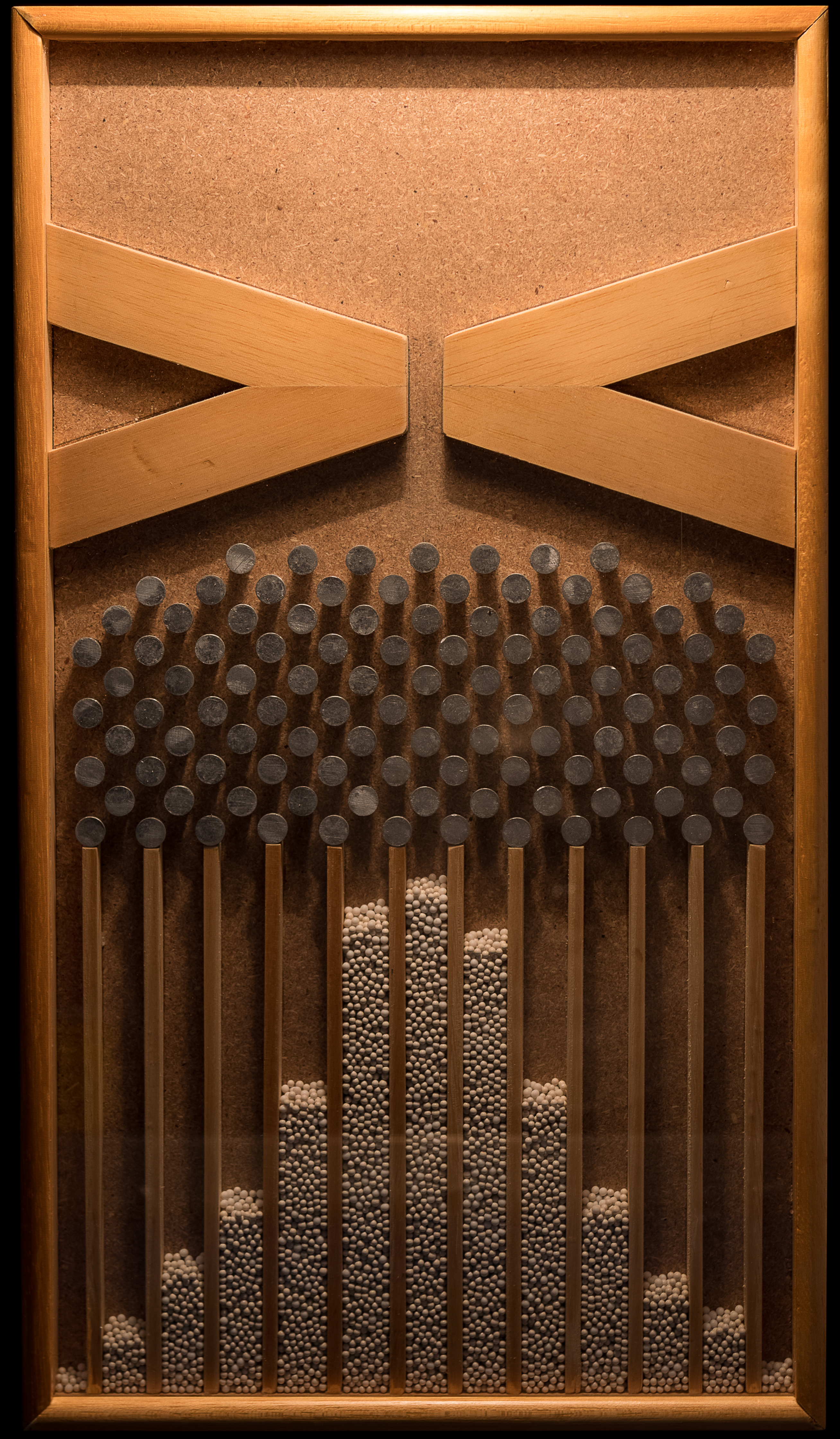
. . .
makeplot <- function() {
  animation::quincunx(balls = 200, col.balls = rainbow(200))
}
gifski::save_gif(makeplot(), "/tmp/galton.gif", 700, 500, delay=0.1)
. . .
Computational notebooks
Render Rmarkdown files
rmarkdown::render('in_class3.Rmd')
Cmd-line:
Rscript -e "rmarkdown::render('in_class3.Rmd')"