CSE 422: Assignment #2

Problem 1: Similarity metrics

You will look at various similarity measures and think about their relative merits. You will need the “20 newsgroups” dataset. Note that newsgroups were part of usenet, which was like reddit but existed even before the internet! (I used it as far back as 1993!)

Each article in the data set is represented as a “bag of words” as follows. There is a list $w_1, w_2, \ldots, w_N$ of all the words occurring in the total collection of documents. To each document $D$, we associate a vector whose $i$th coordinate contains the number of occurrences of $w_i$ in $D$. (Note that the article ids correspond to real articles, but our data set only contains the word frequencies.)

The data is contained in newsgroup_data.yaml. This YAML file contains data in the format

newsgroup_name:
  article_id:
    word_id: count
    word_id: count
    word_id: count
    ...
  article_id:
    word_id: count
    word_id: count
    ...

So, for instance, the following would represent that the newsgroup alt.science contains articles 3 and 7, and article 3 contains 2 occurrences of word 1, 14 occurrences of word 2, 2 occurrences of word 5, and 7 occurrences of word 9.

alt.science:
  3:
    1: 2
    2: 14
    5: 2
    9: 7
  7:
    1: 2
    4: 4
    5: 2
    10: 7

Note that, while there are many words, any particular document probably contains only a small set of them. Thus it makes sense to represent only the non-zero entries of the vector.

You will explore the following similarity metrics, where $\mathbf{x}$ and $\mathbf{y}$ are two bag-of-words vectors:

• Jaccard similarity: \[ J(\mathbf{x},\mathbf{y}) = \frac{\sum_i \min(x_i,y_i)}{\sum_i \max(x_i,y_i)} \]
• $L_2$ similarity: \[ L_2(x,y) = - \|\mathbf{x}-\mathbf{y}\|_2 = - \sqrt{\sum_i |x_i-y_i|^2} \]
• Cosine similarity: \[ S_C(x,y) = \frac{\sum_i x_i \cdot y_i}{\|\mathbf{x}\|_2 \|\mathbf{y}\|_2} \]

Note that the Jaccard and cosine similarity are numbers in the interval $[0,1]$, while the $L_2$ similarity (which is the negative of the Euclidean distance) lies in $(-\infty,0]$. We have arranged so that larger numbers represent more similarity.

(a) [8 points]

Implement each of the similarity metrics above and for each metric. For each one, you will prepare a heat map. Here’s an example:

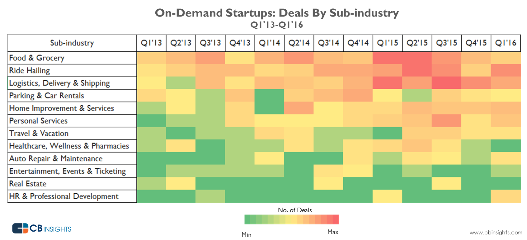
See this python code for an example of how to create heat maps with pyplot.

Your plot will be a $20 \times 20$ matrix with rows and columns indexed by newsgroups (in the same order). For each entry $(A,B)$ of the matrix, compute the average similarity over all ways of pairing up one article from $A$ with one article from $B$. After computing these $400$ numbers, plot your results in a heat map.

Make sure to label your axes with the group names and choose an appropriate colormap. (The idea is that the colors should have a natural, intuitive interpretation as similar vs. dissimilar.) Make sure to give a legend (as in the figure above) to indicate what the colors mean.

Submit your heat maps and paste your code into the typeset assignment.

(b) [4 points]

Based on your three heatmaps, which similarity measure(s) seems the best or worst? Can you explain why this might be the case? Are there pairs of newsgroups that appear very similar? Can you explain why?

Submit your explanation and discussion.

Problem 2: Dimension reduction

You may have noticed that it takes a non-trivial amount of time to compujte pairwise distances for Problem 1. You will implement a dimension-reduction method to reduce the running time. In the following, $k$ will refer to the original dimension of your data and $d$ will refer to the target dimension.

(a) [3 points] Baseline classification

Implement a baseline cosine-similarity nearest-neighbor classification system that, for any given document, finds the document with largest cosine similarity and returns the corresponding newsgroup label. You should use brute-force search.

Compute the $20 \times 20$ matrix whose $(A,B)$ entry is defined by the fraction of articles in group $A$ that have their nearest neighbor in group $B$. Plot the results using a heat map as in Problem 1.

What is the average classification error (i.e., what fraction of the 1000 articles don’t have the same newsgroup label as their closest neighbor)?

Submit your heat maps, code, and classification error.

(b) [2 points]

Your plots for Part 1(b) were symmetric. Why is the matrix in (a) not symmetric?

(c) [3 points]

There is a famously flawed study which shows that certain behaviors (e.g., smoking, obesity) are contagious along social networks. One of the obstacles such a study faces is in explaining how the results arise from causation (being friends with an obese person makes you more likely to be obese) rather than correlation (e.g., common environmental factors—like the quality of easily accessible cheap food).

The authors used data in which people name their close friends. For two people $A$ and $B$, let us write $A\to B$ if $A$ named $B$ as a friend, but $B$ did not name $A$. And write $A \leftrightarrow B$ if they named each other. The authors of the study noticed that if $A \leftrightarrow B$ then the correlation of various properties was higher than if only $A \to B$. They used this (and related properties) to argue in favor of causation.

For documents $A$ and $B$, let us write $A \to B$ if $B$ is the nearest neighbor to $A$, but $A$ is not the nearest neighbor to $B$. Write $A \leftrightarrow B$ if $A$ and $B$ are nearest-neighbors to each other. Let $\mathcal{D}_1 = \{ (A,B) : A \to B \}$ and $\mathcal{D}_2 = \{(A,B) : A \leftrightarrow B \}$. Use your data structure to compute the average similarity of articles $A,B$ as $(A,B)$ ranges over $\mathcal{D}_1$, and the average similarity of articles as $A,B$ as $(A,B)$ ranges over $\mathcal{D}_2$. Report these two numbers.

Submit your code and average similarity values.

(d) [2 points]

Discuss how the values you found might explain why pairs of friends with $A \leftrightarrow B$ had higher correlations than those with $A \to B$ without assuming any causation. (If you struggle to come up with an answer, see pages 8-10 here.)

(e) [7 points]

Implement the following random projection algorithm for dimension reduction.

Given a set of $k$-dimensional vectors \( \{v_1,v_2,\ldots,\} \), define a $d \times k$ matrix $M$ by drawing each entry randomly (and independently) from a normal distribution with mean $0$ and variance $1$. The $d$-dimensional reduced vector corresponding to $v_i$ is given by the matrix-vector product $M v_i$. You can think of the matrix $M$ as a set of $d$ random $k$-dimensional vectors \( \{w_1,\ldots,w_d\} \) (the rows of $M$), and then the $j$th coordinate of the reduced vector $M v_i$ is the inner product between $v_i$ and $w_j$. [If needed: A reminder about matrix-vector products.]

Plot the nearest-neighbor visualization (heat map) as in part (a) for $d=10,30,60,120$.

What is the average classification error for each $d$? For which values of the target dimension are the results comparable to the original data set?

Submit your code, heat maps, and classification errors.

(f) [5 points]

Suppose you are trying to build a very fast article classification system and have an enormous data set of $n$ labeled articles. What is the overall asymptotic (Big-$O$) running time of classifying a new article as a function of $n$ (the number of data points), $k$ (the original dimension), and $d$ (the reduced dimension)?

Now suppose you are instead trying to classify tweets so that the bag-of-words representation if still a $k$-dimensional vector, but now each tweet has only $50 \ll k$ words. Explain how you might exploit the sparsity of the data to improve the runtime of the naive system from part (a).

How does this runtime compare to that of a dimension-reduction nearest-neighbor system (as in part (e)) that reduces the dimension to $d=50$? [We want a theoretical discusison here; there is no need to run code for this part.]

ExtraCredit 2EC: Analysis of minHash embedding [math, 6 pts]

In the curse of dimensionality lecture notes, I claim that for a value \(\ell \leq O(\frac{\log n}{\e^2})\) and any set of \(n\) users, with high probability, the dimension-reduced distance \(J^H\) is a \((1 \pm \e)\)-approximation to the original distance for all \(n\) users. Use the following Bernstein inequlaity to prove this claim formally.

Bernstein’s inequality: Suppose that \(X_1,\ldots,X_n\) are independent random variables with \(\E[X_i]=0\) for \(i=1,2\ldots,n\), and that we have an absolute upper bound \(|X_i| \leq M\) for \(i=1,\ldots,n\). Then for all \(t > 0\), it holds that