Consider a function \(f : \R^n \to \R_+\) that can be written as a sum of a large number
of functions \(f = f_1 + f_2 + \cdots\) from some class. When can this sum be
sparsified in the sense that f can be approximated by a (nonnegative) weighted
combination of a small number of the \(\{f_i\}\)? For many classes of functions, the
answer is that, surprisingly, only about \(O(n)\) summands suffice (up to
logarithmic factors). When this is possible, one can address the algorithmic
questions: How to efficiently construct the sparsifier, and how to use sparse
representations to optimize \(f\) efficiently.
This simple question has a wealth of applications in CS (especially in big
data analysis), as well as in many areas of mathematics (especially in
functional analysis and convex geometry). The course will focus on the
mathematical structures underlying sparsification problems, covering
things like: Leverage scores, Lewis weights, generalized linear regression,
spectral sparsification of graphs, matrix concentration, generic chaining
theory, subspace embeddings and dimension reduction, submodularity, and
low-rank approximation in numerical linear algebra.
Consider the prototypical problem of least-squares linear regression: Suppose we are given input pairs
\((a_1,b_1), (a_2,b_2) \ldots, (a_m,b_m)\) with \(a_1,\ldots,a_m \in \R^n\) and \(b_1,\ldots,b_m \in \R\),
and we want to find \(x \in \R^n\) such that \(\langle a_i,x\rangle \approx b_i\) for all \(i=1,\ldots,m\).
Let \(A\) be the \(m \times n\) matrix whose rows are \(a_1,\ldots,a_m\).
We will assume that the data is noisy and the system is overdetermined (\(m \gg n\)) so that there is no actual solution to \(Ax=b\).
In this case, a natural thing to try is to minimize the least-squares error:
\[\textrm{minimize}\ \left\{ \|Ax-b\|_2^2 : x \in \R^n \right\}.\]
One might now ask the question of whether we really need to work with all \(m\) examples
given that the dimensionality is only \(n \ll m\). Here’s one possible formulation of this problem:
Is there a matrix \(\tilde{A}\) with \(\tilde{m} \approx n\) rows and such that the solution
to any least-squares regression problem with \((\tilde{A},b)\) is close to the solution with \((A,b)\)?
Even more ambitiously, we could ask that every row of \(\tilde{A}\) is a weighted scaling of some row of \(A\).
Thus \(\tilde{A}\) would correspond to the weighted input \(c_{i_1} (a_{i_1}, b_{i_1}), c_{i_2} (a_{i_2}, b_{i_2}), \ldots, c_{i_M} (a_{i_M}, b_{i_M})\),
with \(c_{i_1}, c_{i_2}, \ldots \geq 0\),
and the property we’d like to have is that \(\|A x - b\|_2 \approx \|\tilde{A} x - b\|_2\) for every \(x \in \R^n\).
Sparsification
This is a special case of a general type of sparsification problem: Suppose that $F : \R^n \to \R_+$ is given by
for some nonnegative weights \(c_1,c_2,\ldots,c_m \geq 0\). Say that the representation is \(s\)-sparse if at
most \(s\) of the weights are nonzero. Say that \(\tilde{F}\) is an \(\e\)-approximation to \(F\) if it holds that
\[|F(x)-\tilde{F}(x)| \leq \e F(x),\quad \forall x \in \R^n\,.\]
General linear models
Our least-squares regression problem corresponds to the case where \(f_i(x) = \abs{\langle a_i,x\rangle - b_i}^2\) for \(i=1,\ldots,m\).
$\ell_p$ loss. But one can imagine many other loss functions. If, instead, we took \(f_i(x) = \abs{\langle a_i,x\rangle - b_i}^p\), the corresponding
problem is called $\ell_p$ regression. Jumping ahead:
It is known that for \(p=1\), there are \(s\)-sparse \(\e\)-approximations with \(s \leq O(\frac{n}{\e^2} \log n)\). [Tal90]
For \(1 < p < 2\), there are \(s\)-sparse \(\e\)-approximations with \(s \leq O(\frac{n}{\e^2} \log n (\log \log n)^2)\).
[Tal95]
For \(0 < p < 1\), there are \(s\)-sparse \(\e\)-approximations with \(s \leq O(\frac{n}{\e^2} (\log n)^{3})\).
[SZ01]
For \(p > 2\), it must be that \(s\) grows like \(n^{p/2}\) (and this is tight).
[BLM89]
Moreover, for \(p = 2\), a remarkable fact is that one can do even better: \(s \leq O(n/\e^2)\).
[BSS14]
In general, one can ask the question: Suppose that \(f_i(x) \seteq \varphi(\langle a_i,x\rangle - b_i)\).
For what loss functions \(\varphi : \R \to \R_+\) is such sparsification possible?
Huber and \(\gamma_p\) losses.
An interesting example is the Huber loss where \(\varphi(y) = \min(y^2, |y|)\). (The Huber
loss is more general, but this special case captures its essence.)
The loss function grows quadratically near \(0\), but is much less sensitive to outliers than the \(\ell_2\) loss.
In general, functionals that grow like \(\varphi(y) = \min(y^2, |y|^p)\) for \(0 < p \leq 2\) have been studied,
especially in the context of fast algorithms for solving \(\ell_p\) regression to high accuracy (see, e.g., [BCLL17]).
The best published work achieves \(s \leq O(n^{4-2\sqrt{2}})\) [MMWY21], but we will see, using methods in this course (from
upcoming joint work with Jambulapati, Liu, and Sidford) that \(s \leq O(\frac{n}{\e^2} (\log n)^{O(1)})\) is possible.
What about the function \(\varphi(y) = \min(y^2, 1)\)? This is sometimes called the Tukey loss,
where we know only partial answers to the sparsification question.
ReLUs. For an example of a loss function that doesn’t allow sparsification, consider \(\varphi(y) = \max(0, y - 0.5)\).
The functional \(f_i(x) = \max(0, \langle a_i,x\rangle - 0.5)\) “lights up” only when \(\langle a_i,x\rangle\) is substantial.
But one can easily choose exponentially many unit vectors \(\{a_i\}\) in \(\R^n\) where these functionals have disjoint support,
meaning that there is no way to sparsify down to fewer than a number of terms that’s exponential in the dimension.
If we choose \(f_i(x) = \max(0, |\langle a_i,x\rangle| - 0.5)\), then \(f_1,\ldots,f_m\) are symmetric and convex, so those
two conditions alone are not enough to give strong sparsification.
In general, we don’t yet a complete theory of sparsification even for 1-dimensional functions.
Graph sparsification
Consider an undirected graph \(G=(V,E,w)\) with nonnegative weights \(w : E \to \R_+\) on the edges.
Let us enumerate the edges of \(G\) as \(u_1 v_1, u_2 v_2, \ldots, u_m v_m\), and define
\(f_i(x) = w_{u_i v_i} |x_{u_i} - x_{v_i}|\). Then,
and for \(x \in \{0,1\}^V\), the latter sum is precisely the total weight of the edges
crossing the cut defined by \(x\).
Now the question of whether \(F\) admits an \(s\)-sparse \(\e\)-approximation is precisely the
question of whether the weighted graph \(G\) admits a cut sparsifier in the sense of Benczur and Karger.
If we instead define \(f_i(x) = w_{u_i v_i} |x_{u_i}-x_{v_i}|^2\), then the question becomes one
about spectral graph sparsifiers in the sense of Spielman and Teng.
High-dimensional sparsification
Hypergraph cut sparsifiers. Suppose now that \(H=(V,E,w)\) is a weighted hypergraph in the sense that each hyperedge \(e \in E\)
is a subset of vertices. If we define, for \(e \in E\),
Symmetric submodular functions. More generally, we can ask about the setting where \(f_1,\ldots,f_m : \R^n \to \R_+\) are symmetric submodular functions
and
(More precisely, one should take each \(f_i\) to be the Lovasz extension of a symmetric submodular function with \(f_i(\emptyset) = 0\).)
For \(p=1\), this generalizes the setting of hypergraph cut sparsifiers,
and one can achieve \(s \leq \frac{n}{\e^2} (\log n)^{O(1)}\).
For \(p=2\), the best-known bound is \(s \leq \frac{n^{3/2}}{\e^2} (\log n)^{O(1)}\), and it’s unknown whether one can do better.
General submodular functions. For more general (non-symmetric) submodular functions, there are many classes
of functions that allow varying degrees of sparsification. See, e.g., [KK23].
Unbiased estimators and importance sampling
Unbiased estimators. A general method to construct sparsifiers is by independent random sampling. Suppose we are in the setting \eqref{eq:F} and
let \(\rho = (\rho_1,\ldots,\rho_m)\) be a probability vector, i.e., a nonnegative vector with \(\rho_1 + \cdots + \rho_m = 1\).
Let us sample indices \(i_1,i_2,\ldots,i_M\) i.i.d. from \(\rho\) and define the random sparsifier \(\tilde{F}\) by
and therefore \(\E[\tilde{F}(x)] = F(x)\) as well.
Importance. As we just argued, \(\tilde{F}(x)\) is an unbiased estimator for any \(\rho\), but crucially in order to choose \(M\) small
and still hope that \(\tilde{F}\) will be a good approximation to \(F\), we need to choose \(\rho\) carefully.
A simple example comes from the \(\ell_2\) regression problem. Let us assume that \(b=0\) and consider \(a_1,\ldots,a_m \in \R^n\) such that \(a_1\) is linearly
independent from \(a_2,\ldots,a_m\). Then \(f_1(x) = |\langle a_1,x\rangle|^2\) must appear in a sparse approximation to \(F\) to handle the input \(x = a_1\).
Therefore we will need to sample at least \(O(1/\rho_1)\) terms before we expect to have \(f_1\) appear.
If we are looking to have \(M \leq n (\log n)^{O(1)}\), it’s clear that choosing \(\rho\) to be uniform, for instance, will be drastically insufficient.
Concentration. In general, once we choose \(\rho\), we are left with the non-trivial problem of getting \(F(x) \approx \tilde{F}(x)\)
for every \(x \in \R^n\). This can be a daunting task that is often framed as bounding an expected maximum:
\(\ell_2\) regression and statistical leverage scores
Considering \(F(x) = f_1(x) + \cdots + f_m(x)\), one way to choose an importance for each \(f_i\) is to obtain
a uniform bound on each term. In other words, we consider the quantity
\[\alpha_i \seteq \max_{0 \neq x \in \R^n} \frac{f_i(x)}{F(x)}\,.\]
If we assume that \(F\) and \(f_i\) scale homogeneously (e.g., in the case of \(\ell_2\) regression, \(F(\lambda x) = |\lambda|^2 F(x)\) and
similarly for each \(f_i\)), then we can write this as
for \(a_1,\ldots,a_m \in \R^n\), and we define \(A\) as the matrix with \(a_1,\ldots,a_m\) as rows.
We’ll derive our importance scores in a few different ways. Each of these perspectives will be useful
for moving later to more general settings.
Uniform control.
Consideration of \eqref{eq:uniform-con} in this setting is easy:
therefore our corresponding sample probabilities would be \(\rho_i \seteq \sigma_i(A)/\mathrm{rank}(A)\).
We will assume in the rest of this lecture that \(\mathrm{rank}(A) = n\), but this is only for convenience.
Symmetry considerations.
We have already seen that if \(a_1\) is linearly independent
from the rest of the vectors, then we should sample it with a pretty large probability (considering the case where \(a_1,\ldots,a_n\)
forms an orthonormal basis, “large” will have to mean probability \(\approx 1/n\)).
Another indication comes from how \(F\) scales: If we replace \(a_1\) by two copies of \(a_1/\sqrt{2}\), then the function \(F\) doesn’t change.
This suggests that \(\rho_i\) should scale proportional to \(\|a_i\|_2^2\).
But notice also that \(F\) is a sum of squares; as there are no cancellations, it is natural to consider
the matrix \(a_1 a_1^{\top} + \cdots + a_m a_m^{\top} = A^{\top} A\). Let’s suppose, for simplicity, that
the vectors form a decomposition of the identity:
Then we have \(\|a_1\|_2^2 + \cdots + \|a_m\|_2^2 = \tr\left(a_1 a_1^{\top} + \cdots + a_m a_m^{\top}\right) = \tr(I) = n\), so symmetry suggests
we take \(\rho_i \seteq \|a_i\|_2^2/n\).
For the general case, let us assume that \(A\) has full rank, i.e., \(\mathrm{rank}(A) = n\).
We can left-multiply the vectors by \((A^{\top} A)^{-1/2}\) to achieve \eqref{eq:isotropic}, again suggesting the
probabilities \(\rho_i = \sigma_i(A)/n\).
We can think about leverage scores in a couple of other ways.
Expected contribution to \(F(x)\).
One way to judge the importance of \(a_i\) is to switch from a “worst case” perspective (approximating \(F(x)\) for every \(x\))
to an ``average case’’ one: Suppose that \(\mathbf{X}\) is a random vector in \(\R^n\) and define
What distribution should we use? In the case that \eqref{eq:isotropic} holds, it makes sense for \(\mathbf{X}\) to be rotationally
invariant, and indeed any such choice works. Using the Gaussian measure on $\R^n$, this would give
and it is straightforward to check that \(\rho_i \propto \|a_i\|_2^2\). And if we apply the
transformation \((A^{\top} A)^{-1/2}\) to a general set of vectors to achieve \eqref{eq:isotropic}, then the corresponding
form is
and again one has \(\rho_i \propto \|(A^{\top}A)^{-1/2} a_i\|_2^2\).
Singular value decomposition.
Suppose we write \(A = U \Sigma V^{\top}\). Recall that we consider \(n \leq m\), thus \(\Sigma = \begin{bmatrix} D \\ \hline 0\end{bmatrix}\),
where \(D\) is an \(n \times n\) diagonal matrix containing the singular values \(\sigma_1,\ldots,\sigma_n\).
Note that \(U\) is an \(m \times m\) matrix, but \(\Sigma\) makes all but the first \(n\) columns of \(U\) meaningless (indeed,
one can obtain an SVD from any completion of the first \(n\) columns of \(U\) to an orthonormal basis).
If we consider the “compact SVD” \(A = \hat{U} \Sigma V^{\top}\) where we cut the last \(m-n\) columns off of \(U\), then \(\sigma_i(A) = \|\hat{u}_i\|_2^2\),
where \(\hat{u}_1,\ldots,\hat{u}_m\) are the rows of \(\hat{U}\).
Concentration
Once we’ve chosen our sampling probabilities \(\rho_i = \sigma_i(A)/n\), we can independently sample \(M\) terms
from the distribution, and we are left to analyze the random sum
We have already argued that \(\E[\tilde{A}] = A\), so the real question is about concentration, which we will begin to cover
in the next lecture.
There are actually two ways to approach this question. One is to think about proving concentration of the sum along every direction \(x \in \R^n\)
simultaneously. This leads naturally to entropy bounds, covering numbers, and the generic chaining theory.
The second approach is to think about \(\tilde{A}\) as a random operator and try to prove concentration of sums of independent random matrices.
The former will be far more general, while the latter appears substantially more powerful in certain special cases.
Recall that we have a function \(F : \R^n \to \R\)
written as \(F(x) = f_1(x) + \cdots + f_m(x)\) and we want to sparisfy it by
sampling the terms in proportion to a probability vector \(\rho \in \R_+^m\) (the “importance scores”).
One way to analyze this is to first make sure all the probabilities are uniformly small, say \(\rho_1,\ldots,\rho_m \leq 2/m\).
Since we are trying to sparsify down to a number of terms that is independent of \(m\), we can always achieve
this by simply splitting a term
Then one can sparsify in phases by deleting every term independently with probability \(1/2\). This experiment can be modeled
with \(\{0,1\}\) random variables in the natural way:
where \(\e_1,\ldots\e_m\) are i.i.d. uniform random $\pm 1$ variables, and \(\Omega \subseteq \R^n\) is our domain of interest.
It turns out that it is possible to do something similar and reduce the analysis of one-shot sampling
to the analysis of randomly signed sums of the functions. This makes for both a simpler algorithm,
and a more robust method of analysis that will be very useful later.
Symmetrization, take II
Let’s consider a more general situation. Consider a family of independent random functions \(\mathbf{g}_1,\ldots,\mathbf{g}_M : \R^n \to \R\)
that are sampled from some distribution. (Recall that we are thinking about each one as being chosen from a finite family of functions and, in our case,
it even holds that they are i.i.d.).
Define \(\mathbf{G}(x) \seteq \mathbf{g}_1(x) + \cdots + \mathbf{g}_m(x)\) and \(F(x) \seteq \E[\mathbf{G}(x)]\).
We are interested in the quantity
where \(\delta < 1\). Then we have \(\mathcal{S} \lesssim \delta\).
Proof: Note that if \(\tilde{\mathbf{g}}_1, \ldots, \tilde{\mathbf{g}}_M\) is an independent family of functions from the same distribution, then
clearly \(F(x) = \E\left[\tilde{\mathbf{g}}_1(x) + \cdots + \tilde{\mathbf{g}}_M(x)\right]\) as well, so we can write
and note that since \(\mathbf{g}_i(x) - \tilde{\mathbf{g}}_i(x)\) and \(\tilde{\mathbf{g}}_i(x)-\mathbf{g}_i(x)\) have the same distribution, we can write this as
Given the above discussion and recalling the definition in \eqref{eq:Esup}, if \eqref{eq:rad} holds for every choice of \(g_1,\ldots,g_M\), this yields the bound
where the last inequality uses concavity of the square root to move the expectation inside.
For \(\delta < 1\), this tells us that \(\mathcal{S} \leq O(\delta)\).
This completes the symmetrization argument, allowing us to focus on proving bounds like \eqref{eq:rad}.
The advantage here lies in the the fact that \(\left \{ \e_1 g_1(x) + \e_2 g_2(x) + \cdots + \e_M g_M(x) : x \in \R^n \right\}\)
is an example of a subgaussian process, and bounding the expected maximum of a subgaussian process has a long and rich history,
along with a correspondingly powerful framework.
The (mild) disadvantage is that we require the inequality \eqref{eq:rad} to hold for every choice of functions \(g_1,\ldots,g_M\)
in the support of our distribution.
(Note: The confusing terminology “process” is a historical artifact. Originally,
one was indeed interested in \(\e_1 g_1(x)\), \(\e_1 g_1(x) + \e_2 g_2(x)\), etc. as a sequence “evolving in time.”
If one switches from discrete to continuous time, e.g., a process like Brownian motion, then control of the
expected maximum is closely related to almost sure continuity of the sample paths.)
Subgaussian processes
Consider a collection of random variables \(\{ X_t : t \in T \}\) where the index set \(T\) is
equipped with a distance \(d\).
The family is called subgaussian (with respect to \(d\)) if there
if there is a constant \(c > 0\) such that
Gaussian processes. The canonical example occurs when \(\{X_t : t \in T\}\) is a jointly Gaussian family of random variables,
in which case \eqref{eq:subgaussian} holds with \(c=1/2\) and \(d(s,t) = (\E |X_s-X_t|^2)^{1/2}\).
Note that if the index set \(T\) is finite, then such a family can always be realized in the following way:
Let \(g_1,g_2,\ldots,g_m\) be i.i.d. \(N(0,1)\) random variables and define
\(X_t = t_1 g_1 + t_2 g_2 + \cdots + t_m g_m\) for \(t \in T \subseteq \R^n\).
Bernoulli processes. Suppose that \(\e_1,\ldots,\e_m\) are i.i.d uniform \(\pm 1\) random variables and for \(t \in T\), we define
\(X_t \seteq \e_1 t_1 + \e_2 t_2 + \cdots + \e_m t_m\). Then the \(\{ X_t : t \in \R^n \}\) is a family
of subgaussian random variables with the same parameters: \(c=1/2\) and \(d(s,t) = (\E |X_s-X_t|^2)^{1/2}\).
Many proofs are known. Even proofs of significant generalizations can be made quite short. See, e.g., the proof of Theorem 1.3 here.
The quantity we care about after our symmetrization argument is
and as we have just seen this is the expected maximum of a centered subgaussian process. (Centered means that \(\E X_t = 0\) for every \(t \in T\).)
There is a rich history and theory for
bounding such expected maxima, with M. Talagrand as the primary architect (see his comprehensive book on the topic).
Suppose now that \(\{ X_t : t \in T \}\) is subgaussian with respect to the distance \(d\).
Our goal is to get some control on \(\E \max_{t \in T} X_t\), and one of the central tenants
of the theory is that we can do this using just the geometry of the distance \(d\).
Let’s suppose that \(d\) is symmetric \(d(s,t)=d(t,s)\) for all \(s,t \in T\), and that it
satisfies the triangle inequality:
Define the quantity \(e_h(T,d)\) as the smallest radius \(r\) such that \((T,d)\) can be
covered by at most \(2^{2^h}\) balls of radius \(r\), where a ball in \((T,d)\) is given by
\[B(t, r) \seteq \{ s \in Y : d(s,t) \leq r \}\,.\]
It follows by a greedy construction
that there exists a “net” \(N_h \subseteq T\) such that \(|N_h| \leq 2^{2^h}\) and
every point of \(T\) is within distance at most \(e_h(T,d)\) of a point in \(N_h\).
It is useful to think of \(N_h\) as the “best” uniform approximation of \((T,d)\) when
one is only allowed to use \(2^{2^h}\) points.
Let’s fix any such sets \(\{N_h : h=0,1,2,\ldots\}\).
Let \(\pi_h : T \to N_h\) be a map that satisfies
\[\begin{equation}\label{eq:pih}
d(t, \pi_h(t)) \leq e_h(T,d)\,\qquad \forall t \in T\,.
\end{equation}\]
For instance, a natural choice is for \(\pi_h(t)\) to map \(t\) to the closest point of \(N_h\),
but we will only need \eqref{eq:pih}.
If we think about \(U_h\) as containing “edges” that gets stretched to random lengths,
then this event entails no edge of \(U_h\) being stretched too much.
Since every pair in \(U_h\) is within distance \(2 e_h(T,d)\), a union bound combined with \eqref{eq:subgaussian} gives
where we have used the obvious bound \(\abs{U_h} \leq \abs{N_h} \abs{N_{h+1}}\) and the fact that \(\abs{N_h} \abs{N_{h+1}} \leq 2^{2^h} 2^{2^{h+1}}\).
A natural choice is now \(\lambda \seteq 4 \frac{\alpha}{c} 2^{h/2}\) for some number \(\alpha > 0\) we will choose later.
If we define \(\mathcal{E}_h \seteq \mathcal{E}_h((\alpha/c) 2^{(h+2)/2})\), then the preceding bound gives us
Note that the leading constant is not so important, we just wanted a clean form for the lower bound. The
real point here is that \(\lambda\) is scaling like \(2^{h/2}\), and the probability of \(\mathcal{E}_h\)
not occurring can be summed over all \(h \geq 0\), since it’s doubly geometric.
If we now simply take a union bound over \(h=0,1,2,\ldots,\), we get
We’ve gone through all this effort because it turns out that if \(\mathcal{E}_h\) holds for every \(h \geq 0\), it gives
us a bound on \(\E \max_{t \in T} (X_t - X_{t_0})\), where \(\{t_0\} = N_0\) (note that \(N_0\) could be any fixed point of \(T\)).
The argument goes via chaining. Consider first the infinite telescoping sum
If we think of this as a chain, then every link in the chain is going to lie in some set \(U_h\), and thus having
control on the stretch of all the “edges” we considered previously will give us control on every term in this chain.
You can assume the sum is finite if you like, because
which goes nicely with our goal of bounding \eqref{eq:delta-bound} via \eqref{eq:dudley}.
Bounding the entropy numbers.
For a metric space \((T,d)\), define \(\mathcal{N}(T,d,\e)\) as the minimal number of \(\e\)-balls
in \((T,d)\) needed to cover \(T\).
It will help to check one’s understanding of the definitions to verify that if
where \(B_2^n\) is the unit ball in the Euclidean norm.
Sparsifiers for \(\ell_2\) regression.
Let us first use the Covering Lemma to finish our first construction of sparsifiers for \(\ell_2\) regression.
Recall that we choose \(\rho_{i} \seteq \|(A^{\top} A)^{-1/2} a_i\|_2^2/n\), where \(A\) is the matrix
with rows \(a_1,\ldots,a_m\) and, in this case, \(F(x) = \|Ax\|_2^2\).
Using the linear transformation \(x \mapsto (A^{\top} A)^{-1/2} x\), we can write
where \(U\) is the matrix with rows \(u_j \seteq \frac{(A^{\top} A)^{-1/2} a_{\nu_j}}{\sqrt{M \rho_{\nu_j}}}\).
Note that, by our choice of \(\rho_1,\ldots,\rho_M\), we have
where the last inequality holds for the unit ball of any norm on \(\R^n\) (and, indeed, \(d_{\nu,\infty}\)
is a distance induced by a norm on \(\R^n\)), as you show in Homework #1.
Putting everything together. Now \eqref{eq:ent1} and \eqref{eq:ent2} in conjunction give
Therefore by setting \(M \seteq C \frac{n}{\e^2} (\log n)^2 \log(n/\e)\) for an appropriate constant \(C > 1\),
\eqref{eq:Fapprox} gives us our desired \(\e\)-approximation.
The covering lemma
Before proving the lemma, it helps to consider the more basic problem of covering the Euclidean
ball \(B_2^n\) by translates of \(\e B_{\infty}^n\), i.e., by translates of small cubes.
Suppose \(\|x\|_2^2 = x_1^2 + x_2^2 + \cdots + x_n^2 = 1\). Since we only care about approximation
up to \(\e\) in the \(\ell_{\infty}\) distance, we could discretize this vector to lie in, say,
\(\e \mathbb{Z}^n \cap B_2^n\).
The most basic kind of vector we need to cover is of the form
\((0, \pm \e, 0, 0, \pm \e, 0, \pm \e, 0, \ldots, 0)\). Because \(\|x\|_2^2 = 1\), there
are only \(n^{O(1/\e^2)}\) choices for such a vector.
But we also need to handle vectors of the form \((0, \pm 2\e, 0, 0, \pm \e, 0, \pm 2\e, 0, \ldots, 0)\), and so on.
It is not hard to convince one’s self that there are asymptotically fewer vectors of this form.
Ineed, if some entry is \(2\e\) then there are \(n\) choices for where it goes, but there are \(n(n-1)/2\) choics
for where two copies of \(\e\) go. Thus the total number of centers one needs is only \(n^{O(1/\e^2)}\).
Now suppose we wanted to cover \(B_2^n\) instead with cubes of different side lengths, or with parallelpipeds
(where the sides are no longer perpendicular), etc. There is a beautiful approach that gives surprisingly good
bounds for cover \(B_2^n\) by translations of an arbitrary symmetric convex body.
(I have heard it credited to Talagrand, or to Pajor and Talagrand.)
The dual-Sudakov approach.
We will prove the following substantial strengthening of this bound.
Suppose that \(d(x,y) = \|x-y\|\) is a distance induced by some norm $\norm{\cdot}$ on \(\R^n\).
Then for every \(\e > 0\),
The last bound is a basic exercise with the gaussian tail, taking a union bound over the \(M\)
gaussian variables \(\{ \langle u_j,\mathbf{g} \rangle : j \in [M] \}\).
Shift Lemma: Suppose that \(\gamma_n\) is the standard gaussian measure on \(\R^n\)
and \(W \subseteq \R^n\) is any symmetric set (\(W = -W\)) and \(z \in \R^n\). Then,
Let \(B \seteq \{ x \in \R^n : \|x\| \leq 1 \}\) denote the unit ball in our given norm.
By scaling, we can assume that \(\e = 2\).
If we cannot cover \(B_2^n\) by \(N\) translates of \(2 B\), then there must exist
\(x_1,\ldots,x_N \in B_2^n\)
such that \(x_1 + B, \ldots, x_N + B\) are all pairwise disjoint.
Let \(\lambda > 0\) be a parameter we will choose momentarily, and note that
\(\lambda (x_1+B),\ldots, \lambda(x_N+B)\) are pairwise disjoint as well, therefore
\[\begin{align*}
1 \geq \gamma_n\left(\bigcup_{i \leq N} \lambda (x_i+B)\right) &= \sum_{i \leq N} \gamma_n\left(\lambda (x_i+B)\right) \\
&\geq \gamma_n(\lambda B) \sum_{i \leq N} e^{-\lambda^2 \|x_i\|_2^2/2} \\
&\geq \gamma_n(\lambda B) N e^{-\lambda^2/2}\,,
\end{align*}\]
where the first inequality uses the Shift Lemma and the second inequality uses \(x_1,\ldots,x_N \in B_2^n\).
Now note that, by Markov’s inequality, \(\E \|\mathbf{g}\| \geq \lambda \gamma_n(\R^n \setminus (\lambda B))\),
thus taking \(\lambda \seteq 2 \E \|\mathbf{g}\|\) gives \(\gamma_n(\lambda B) \geq 1/2\), and we conclude that
Fix \(1 \leq p \leq 2\).
We will now prove that if \(a_1,\ldots,a_m \in \R^n\)
and \(f_i(x) = |\langle a_i,x\rangle|^p\), then the sum
\(F(x) = f_1(x) + \cdots + f_m(x)\) admits \(s\)-sparse \(\e\)-approximations for
$$
s \lesssim \frac{n}{\e^2} \left(\log \frac{n}{\e}\right)^{O(1)},
$$
generalizing what we saw last lecture for \(p=2\).
As we have already seen, this will follow from an estimate of the form
Let \(B_N\) denote the unit ball of \(N\).
Define \(V(r) \seteq \mathrm{vol}_n(r B_N) = r^n \mathrm{vol}_n(B_N)\) so that \(\frac{d}{dr} V(r) = n r^{n-1} \mathrm{vol}_n(B_N)\).
Therefore,
where the latter equality follows from integration by parts.
Let \(\mathbf{Z}\) be a random variable with law \(\mu\), where \(\mu\) has density proportional to \(e^{-\norm{Ax}_p^p}\).
Then the lemma tells us that
Check that in the case \(p=2\), it holds that \(\rho_i = \norm{(A^{\top} A)^{-1/2} a_i}_2^2/n\), i.e.,
the corresponding weights are precisely the statistical leverage scores.
The shift lemma and uniform smoothness
In light of our choice of important scores in \eqref{eq:lp_scores}, we can think of the following setting.
Let \(U\) be a matrix with rows \(u_1,\ldots,u_M \in \R^n\).
Let \(\mathbf{Z}\) be a random variable whose distribution has density proportional to \(e^{-\|A x\|_p^p}\),
and assume that
Note that if \(u_j = a_{\nu_j}/(M \rho_{\nu_j})^{1/p}\), then \(K \leq (\frac{n}{p M})^{1/p}\) using \eqref{eq:rho-alt}.
Our goal now is to bound the covering numbers of the set \(B_A \seteq \{x \in \R^n : \|A x\|_p \leq 1 \}\)
in the metric \(d_{U}(x,y) \seteq \|U(x-y)\|_{\infty}\).
Recall that we did this in the last lecture in the case \(p=2\) using the Shift Lemma for the gaussian measure.
There we used the inequality
For \(1 \leq p \leq 2\), the \(\ell_p\) norm is \(p\)-uniformly smooth with constant \(1\). This reduces to the \(1\)-dimensional inequality (due to Clarkson):
where the first inequality is concavity of \(y \mapsto y^{q}\) for \(0 \leq q \leq 1\), and the second
inequalitiy uses $(u+v)^q \leq u^q + v^q$ for \(0 \leq q \leq 1\) and \(u,v \geq 0\).
Uniform smoothness is a quantative measure of how much the unit ball of a norm lacks “corners.”
Consider the modulus of smoothness
Then \(N\) is \(p\)-uniformly smooth if \(\rho_N(t) \leq O(t^p)\) for all \(t > 0\).
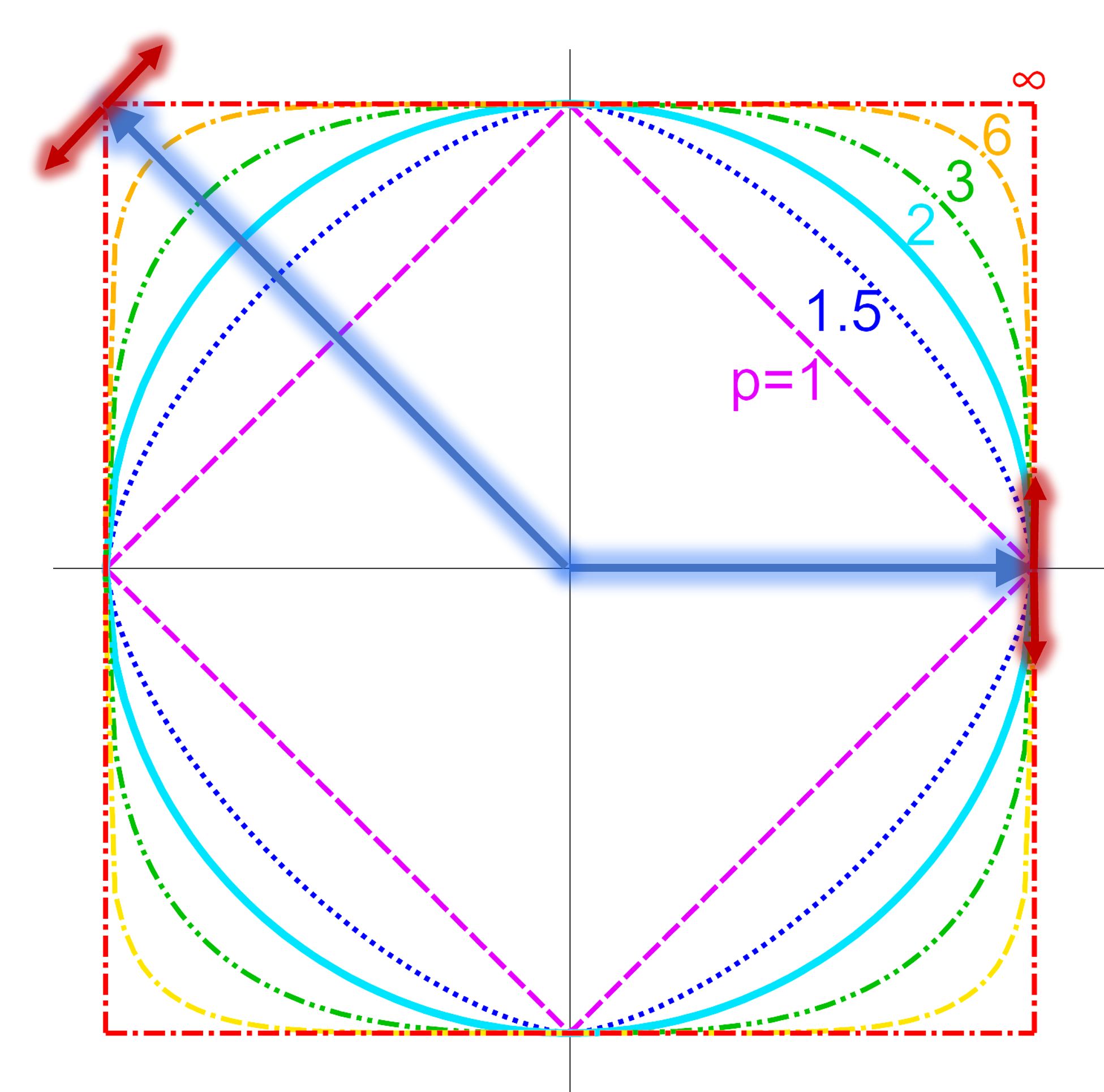
To get some intuition for this notion, see the figure to the right. The blue arrow
corresponds to \(x\) and the red arrows correspond to \(\pm y\). One of the directions
is bad for the \(\ell_1\) ball, and the other for the \(\ell_{\infty}\) ball.
Note how following the red arrows takes one far outside the \(\ell_1\) (and \(\ell_{\infty}\)) ball,
but almost stays inside the \(\ell_2\) ball.
It turns out that \(\ell_p\) is \(p\)-uniformly smooth with constant \(1\) for \(1 \leq p \leq 2\),
and \(2\)-uniformly smooth with constant \(O(\sqrt{p})\) for \(p > 2\).
Shift Lemma for \(p\)-uniformly smooth norms:
Suppose $N$ is a norm on $\R^n$ that is $p$-uniformly smooth with constant $S$. Let \(\mu\)
be the probability measure on \(\R^n\) with density proportional to \(e^{-N(x)^p}\).
Then for any symmetric convex body \(W \subseteq \R^n\) and \(z\in \R^n\),
\[\begin{equation}\label{eq:shift-measure}
\mu(W+z) \geq e^{- S^p N (z)^p}\mu(W)\,.
\end{equation}\]
where the equality uses symmetry of ${W}$, the first inequality uses convexity of $e^y$, and the second inequality
uses $p$-uniform smoothness of $N$ (recall \eqref{eq:p-smooth}).
Dual-Sudakov Lemma for \(p\)-smooth norms.
Let \(N\) and \(\hat{N}\) be norms on \(\R^n\).
Suppose that $N$ is $p$-uniformly smooth with constant $S$,
and let \(\mu\) be the probability measure on $\R^n$ with density
propertional to \(e^{-N(x)^p}\).
Then for any $\e > 0$,
Proof:
By scaling $\hat{N}$, we may assume that $\e = 1$.
Suppose now that $x_1,\ldots,x_M \in B_{N}$ and $x_1+B_{\hat{N}},\ldots,x_M+B_{\hat{N}}$ are pairwise disjoint.
To establish an upper bound on $M$, let $\lambda > 0$ be a number
we will choose later and write
Since it holds that \(\E[\abs{\langle u_j,\mathbf{Z}\rangle}] \leq \left(\E \abs{\langle u_j,\mathbf{Z}\rangle}^p\right)^{1/p} \leq L^{1/p}\) by \eqref{eq:pth-moments},
we are left with the final piece, a concentration estimate for the random variables \(\{ \langle u_j, \mathbf{Z} \rangle \}\).
\(\psi_1\) concentration for one-dimensional marginals of log-concave measures
Exponential concentration. Let’s first summarize the final piece: The function \(e^{-\|Ax\|_p^p}\) is log-concave, meaning
that the random variable \(\mathbf{Z}\) is log-concave. You will prove in HW#2 that the \(1\)-dimensional marginals of such a random variable always satisfy an exponential concentration inequality: For some constant \(c > 0\),
\[\P\left[\abs{\langle u_j, \mathbf{Z}\rangle} \geq t \E[\abs{\langle u_j, \mathbf{Z}\rangle} \right] \leq e^{-c t}\,,\quad t \geq 1\,.\]
Finishing the argument. In particular, this implies that
And using our symmetrization reduction, we should take \(M \asymp \frac{n}{\e^2} (\log (n/\e))^p (\log n)^2\) to obtain an \(\e\)-approximation
with precisely \(M\) terms.
Claim: Suppose that $U_0$ is a maximizer of \eqref{eq:lewis-opt}. Then,
\((U_0^{\top} U_0)^{-1} = A^{\top} W A\,,\) where $W$ is a nonnegative
diagonal matrix with $W_{ii} = \norm{U_0 a_i}_2^{p-2}$ for $i=1,\ldots,m$.
Proof: The method of Langrange multipliers tells us that there is a nonnegative
$\lambda > 0$ such that the maximum is given by a critical point of the
functional
Assuming that $\mathrm{span}(a_1,\ldots,a_m) = \R^n$, it is
straightforward to check that the optimization has a finite, non-zero
maximum, and therefore any maximizer $U_0$ is invertible.
Let us compute the gradient of $G(U)$ with respect to the matrix entries
${ U_{ij} : 1 \leqslant i,j \leqslant n }$. The rank-one update rule
for the determinant says that for invertible $U$,
\[\det(U + u v^{\top}) = \det(U) (1+\langle v, U^{-1} u\rangle)\,,\]
This follows from $U + uv^{\top} = U (I + U^{-1} uv^{\top})$,
$\det(AB)=\det(A)\det(B)$, and
$\det(I + uv^{\top}) = 1 + \langle u,v\rangle$.
As before, the analysis of concentration for importance sampling comes
down to analyzing covering numbers of the set
\(B_{A,p} \seteq \{ x \in \R^n : \|Ax\|_p \leqslant 1 \}\)
in the metric
From \eqref{eq:l2-lp}, we see that the Euclidean ball
\(B_{\rho,2} \seteq \{ x \in \R^n : \norm{U^{-1} x}_2 \leq 1 \}\)
satisfies $B_{A,p} \subseteq B_{\rho,2}$.
Denote the unit ball
\(B_{\rho,\infty} \seteq \{ x \in \R^n : \norm{x}_{\rho,\infty} \leqslant 1 \}\).
Then we can bound
\[\mathcal{N}(B_{A,p}, r B_{\rho,\infty}) \leqslant\mathcal{N}(B_{\rho,2}, r B_{\rho,\infty})\,.\]
If we apply the linear transformation $U^{-1}$ that takes $B_{\rho,2}$
to the standard Euclidean ball $B_2$, then the dual-Sudakov inequality
tells us how to bound the latter quantity:
\[\begin{equation}\label{eq:lewis-ds}
(\log \mathcal{N}(B_{\rho,2}, r B_{\rho,\infty}))^{1/2} \lesssim \frac{n^{1/p}}{r} \max_{i=1,\ldots,m} \frac{|\langle U a_i, \mathbf{g}\rangle|}{\|U a_i\|_2}
\lesssim \frac{n^{1/p}}{r} \sqrt{\log m}\,.\end{equation}\]
Problematically, this bound is too weak to recover \eqref{eq:ldb}. Taking both sides to the $p/2$ power gives
\[\begin{equation}\label{eq:badcover}
(\log \mathcal{N}(n^{1/p} B_{\rho,2}, r B_{\rho,\infty}))^{1/p} \lesssim \frac{n^{1/2}}{r^{2/p}} (\log m)^{p/4}\,.\end{equation}\]
The issue is that the scaling in $r$ is bad unless $p=2$ (compare \eqref{eq:ldb}).
The problem is our use of the worst-case bound
$B_{A,p} \subseteq n^{1/p} B_{\rho,2}$. There is a more sophisticated
way to bound covering numbers in this setting using norm interpolation
and duality of covering numbers (see Ledoux-Talagrand, Prop 15.19).
But the sort of improvement one needs can be summarized as follows: \eqref{eq:badcover}
is bad for $r \to 0$, but it gives a good bound
for $r$ small, but constant. Having covered $B_{\rho,2}$ by translates
of $B_{\rho,\infty}$, we get an improved bound on the inner products
$|\langle a_i,x\rangle|^{2-p}$ in \eqref{eq:lewis-exp}
This, in turn, gives us a better bound on
$\norm{U^{-1} x}_2$, which means that when we want to reduce the radius
from $r$ to $r/2$ (say), we get an improved estimate for the Euclidean
diameter, making the application of \eqref{eq:lewis-ds} stronger.
Computation of the Lewis weights for $p < 4$: A contraction argument
For $p < 4$, it is possible to compute the Lewis weights using a simple
iterative scheme, assuming that one can compute leverage scores. For a
matrix $A$, define the $i$th leverage score by
$\sigma_i(A) \mathrel{\mathop:}=\langle a_i, (A^{\top} A)^{-1} a_i\rangle$.
In this section, if $W$ is a nonnegative $m \times m$ diagonal matrix,
we will use $w \in \R_+^m$ for the vector with $w_i = W_{ii}$
for $i=1,\ldots,m$.
Define
$\tau_i(w) \mathrel{\mathop:}=\langle a_i, (A^{\top} W A)^{-1} a_i\rangle$.
The idea is to recall that for the Lewis weights, we have
$w_i = \norm{U a_i}_2^{p-2}$, hence
Finally, define the vector $\tau(w) \in \R_+^m$ by
$\tau(w) \mathrel{\mathop:}=(\tau_1(w),\ldots,\tau_m(w))$.
Claim: For any $w,w’ \in \R_+^m$, it holds that \(d(\tau(w),\tau(w')) \leqslant d(w,w')\,.\)
Proof: If $w_i \leqslant\alpha w’_i$ for every $i=1,\ldots,m$, then
$W \preceq \alpha W’$ in the PSD (Loewner) ordering. Therefore
$A^{\top} W A \preceq \alpha A^{\top} W’ A$, and finally
$(A^{\top} W’ A)^{-1} \preceq \alpha (A^{\top} W A)^{-1}$, since matrix
inversion inverts the PSD order.
Finally, by definition this yields
$\langle u, (A^{\top} W’ A)^{-1} u\rangle \leqslant\langle u, (A^{\top} W A)^{-1} u \rangle$
for every $u \in \R^m$. In particular,
$\tau_i(w’) \leqslant\alpha \tau_i(w)$ for each $i=1,\ldots,m$.
Note that if $1 \leqslant p < 4$, then $|(p-2)/p| < 1$, and therefore
$\varphi$ is a strict contraction on the space of weights. In
particular, it holds that for $\delta > 0$ such that
$1-\delta = |(p-2)/p|$, and any $w_0 \in \R_+^m$,
Our goal will be to sparification where the terms are
$f_i(x) \mathrel{\mathop:}=N_i(x)^p$ in our usual notation, and
$F(x) = N(x)^p$.
A semi-norm $N$ is nonnegative and satisfies
$N(\lambda x) = |\lambda| N(x)$ and $N(x+y) \leqslant N(x)+N(y)$ for all
$\lambda\in \R$, $x,y \in \R^n$, though possibly
$N(x)=0$ for $x \neq 0$.
Note that, equivalently, a semi-norm is a homogeneous function:
$N(\lambda x) = |\lambda| N(x)$ such that $N$ is also convex.
Examples
Spectral hypergraph sparsifiers. Consider subsets
$S_1,\ldots,S_m \subseteq {1,\ldots,n}$ and
Then sparsifying $F(x) = f_1(x) + \cdots + f_m(x)$ is called
spectral hypergraph sparsification.
More generally, we can consider linear operators
${ A_i \in \R^{d_i \times n} }$ and the terms
$f_i(x) \mathrel{\mathop:}=\norm{A_i x}_{\infty}^2$.
Symmetric submodular functions. A function
$f : 2^V \to \R_+$ is submodular if
\[f(S \cup \{v\}) - f(S) \geqslant f(T \cup \{v\}) - f(T)\,,\quad \forall S \subseteq T \subseteq V, v \in V\,.\]
If one imagines $S \subseteq V$ to be a set of items and $f(S)$ to
be the total utility, then this says that the marginal utility of an
additional item $v \in V$ is non-increasing as the basket of items
increases. As a simple example, consider
$w_1,\ldots,w_n \geqslant 0$ and
$f(S) \mathrel{\mathop:}=\min\left(B, \sum_{i \in S} w_i\right)$.
Here, the additional utility of an item drops to $0$ as one
approaches the “budget” $B$.
A submodular function $f : 2^V \to \R_+$ is symmetric if
$f(\emptyset)=0$ and $f(S) = f(V \setminus S)$ for all
$S \subseteq V$. A canonical example is where $f(S)$ denote the set
of edges leaving a cut $(S, V \setminus S)$ in an undirected graph.
The Lovász extension of a submodular function is the function
$\tilde{f} : [0,1]^V \to \R_+$ defined by
where $\mathbf{S}_x$ is a random set such that $i \in \mathbf{S}_x$
with probability $x_i$, independently for every $i \in V$.
Fact: A function $f : 2^V \to \R_+$ is submodular if and only if
$\tilde{f} : [0,1]^V \to \R_+$ is convex.
Because of this fact, it turns out that a function $f$ is symmetric
and submodular if and only if $\tilde{f}$ is a semi-norm, where we
extend $\tilde{f} : \R^V \to \R_+$ to all of
$\R^V$ via the definition
\[\begin{equation}\label{eq:lov-ext}
\tilde{f}(x) \mathrel{\mathop:}=\int_{-\infty}^{\infty} f(\{ i : x_i \leqslant t \})\,dt\,.\end{equation}\]
Note that if \(x \in \{0,1\}^V\) is such that
$x_i = \mathbf{1}_S(i)$, then we have
\[\tilde{f}(x) = \int_{0}^1 f(\{ i : x_i \leqslant t \}\,dt\,,\]
since $f(\emptyset)=f(V)=0$. Moreover,
\(\{ i : x_i \leqslant t \} = S\) for $0 < t < 1$, hence
$\tilde{f}(x)=f(S)$. So $\tilde{f}$ is indeed an extension of $f$. A
similar argument shows that for $x$ defined this way,
$\tilde{f}(-x)=f(V \setminus S)$.
Lemma: A function $f : 2^V \to \R_+$ is symmetric and submodular
if and only if $\tilde{f}$ is a semi-norm.
Proof:
A semi-norm $\tilde{f}$ is convex, and therefore by the fact above,
$f$ is submodular. Moreover $\tilde{f}(0)=0$ and
$\tilde{f}(x)=\tilde{f}(-x)$ for a semi-norm, so if
$x \in {0,1}^V$ is given by $x_i = \mathbf{1}_S(i)$, then
$f(S)=\tilde{f}(x)=\tilde{f}(-x)=f(V\setminus S)$ and thus $f$ is
symmetric.
Conversely, if $f$ is symmetric and submodular, then
$\tilde{f}(x)=\tilde{f}(-x)$ and $\tilde{f}$ is convex. Moreover,
the defintion \eqref{eq:lov-ext}
shows that $\tilde{f}(cx)=c \tilde{f}(x)$
for $c > 0$, hence $\tilde{f}$ is also homogeneous, implying that
it’s a semi-norm.
Thus the sparsification problem for sums
$F(S) = f_1(S) + \cdots + f_m(S)$ of symmetric submodular functions
${f_i}$ reduces to the sparsification problem for semi-norms:
$\tilde{F}(x) \mathrel{\mathop:}=\tilde{f}_1(x) + \cdots + \tilde{f}_m(x)$.
Importance scores
Let us consider now the sparsification problem \eqref{eq:ns}
for $p=1$.
As we discussed in previous lectures, a reasonable way of assigning
sampling probabilities is to take
for some random variable $\mathbf{Z}$ on $\R^n$, as this
represents the “importance” of the $i$th term $N_i(x)$ under the
distribution of $\mathbf{Z}$.
Let us also recall the notion of approximation we’re looking for:
Given the desired approximation guarantee, it’s natural to simply take
$\mathbf{Z}$ to be uniform on the unit ball
\[B_N \mathrel{\mathop:}=\{ x \in \R^n : N(x) \leqslant 1 \}\,.\]
For the purposes of analysis, it will be easier to take $\mathbf{Z}$ as
the random variable on $\R^n$ with density proportional to
$e^{-N(x)}$, but let us see that gives the same probabilities
\eqref{eq:ns-rhoi}
as averaging uniformly over $B_N$. To compare
the density $e^{-N(x)}$ and the density that is uniform on $B_N$, one
can take $\varphi_1(y)=e^{-y}$ and
\(\varphi_2(y) = \mathbf{1}_{\{y \leqslant 1\}}\) in the next lemma.
Lemma: Suppose that the density of the random variable $\mathbf{Z}$ is
$\varphi(N(x))$ for any sufficiently nice function $\varphi$. Then the
probabilities defined in \eqref{eq:ns-rhoi}
are independent of $\varphi$.
Proof: Define $V(r) \mathrel{\mathop:}=\mathrm{vol}_n(r B_N)$ and note
that $V(r) = r^n \mathrm{vol}_n(B_n)$. Let
$u : \R^n \to \R$ be a homogeneous function, i.e.,
$u(\lambda x) = |\lambda| u(x)$ for all
$\lambda \in \R, x \in \R^n$. Then we have
Recall that \(N(x) = N_1(x) + \cdots + N_m(x)\,,\) and $B_N$ is the unit
ball in the norm $N$. To apply our standard symmetrization/chaining
analysis, define the metric
where $\mathbf{Z}$ is the random variable with density $e^{-N(x)}$. Note
that this applies without any assumptions on $N$ because every norm is
$p$-uniformly smooth when $p=1$.
Recall that in this setting we take
$\rho_i = \frac{1}{n} \mathbb{E}[N_i(\mathbf{Z})]$,
therefore
We are left to prove \eqref{eq:max-ub}.
First, observe that the maximum need only be
taken over indicies $i$ in the set ${ \nu_1,\ldots,\nu_M }$. So we are
looking at the expected maximum of (at most) $M$ random variables. The
claimed upper bound follows immediately (see Problem 2(A) on Homework #2) from an
exponential concentration inequality:
Note that $N_i$ is only a small piece of the norm $N$, so there is
essentially no exploitable relationship between $N_i$ and $\mathbf{Z}$.
Therefore the concentration inequality will have to hold in some
generality.
Log-concave random vector: A random variable $\mathbf{X}$ on $\mathbb{R}^n$ is log-concave if
its density is $e^{-g(x)}\,dx$ for some convex function
$g : \mathbb{R}^n \to \mathbb{R}$.
Isotropic random vector:
A random variable $\mathbf{X}$ on $\mathbb{R}^n$ is isotropic if
$\mathbb{E}[\mathbf{X}]=0$ and
$\mathbb{E}[\mathbf{X} \mathbf{X}^{\top}] = I$.
Lipschitz functions: A function $\varphi: \mathbb{R}^n \to \mathbb{R}$ is $L$-Lipschitz
(with respect to the Euclidean distance) if
\[|\varphi(x)-\varphi(y)\| \leqslant L \|x-y\|_2\,, \quad \forall x,y \in \mathbb{R}^n\,.\]
Lemma [Gromov-Milman]: If $\varphi: \mathbb{R}^n \to \mathbb{R}$ is $L$-Lipschitz and
$\mathbf{X}$ is an isotropic, log-concave random variable, then
\[\begin{equation}\label{eq:kls-tail}
\mathbb{P}\left(|\varphi(\mathbf{X})-\mathbb{E}[\varphi(\mathbf{X})]| > t L\right) \leqslant e^{-c t/\psi_n}\,,\end{equation}\]
where $c > 0$ is an absolute constant and $\psi_n$ is the KLS constant
in $n$ dimensions.
Note that the KLS constant has many definitions that are equivalent up
to a constant factor, and one could take \eqref{eq:kls-tail} as the definition.
See links to related material at the end.
To prove \eqref{eq:ni-con}, first note that our random variable $\mathbf{Z}$
is log-concave because $N(x)$ is a convex function. To make it
isotropic, we define
$\mathbf{X} \mathrel{\mathop:}=A^{-1/2} \mathbf{Z}$, where
$A \mathrel{\mathop:}=\mathbb{E}[\mathbf{Z} \mathbf{Z}^{\top}]$.
We will apply the lemma to the map $\varphi(x) \seteq N_i(A^{1/2} x)$, and we
need only evaluate the Lipschitz constant of $\varphi$.
In Homework #2
problem 4, you show that $\varphi$ is $L$-Lipschitz with
$L \lesssim \mathbb{E}[N_i(\mathbf{Z})]$, yielding \eqref{eq:ni-con}.
when $\mathbf{Z}$ chosen uniformly (according to the volume measure on
$\mathbb{R}^n$) from the unit ball $B_N$.
A first important thing to
notice is that it suffices to sample according to a distribution
$\tilde{\rho}$ that satisfies $\tilde{\rho}_i \geq c \rho_i$ for all $i=1,\ldots,m$ and some constant $c > 0$.
This follows from the way the importances ${\rho_i}$ are used in our
analyses.
and that our sparsification bounds are in terms of entropy numbers $e_{h}(B_F, d_{\nu,\rho})$
with \(B_F \seteq \{ x \in \R^n : F(x) \leq 1 \}\). Note that for an approximation $\tilde{\rho}$ as above, we have
which implies $e_h(B_F, d_{\nu,\tilde{\rho}}) \leq \frac{1}{c} e_h(B_F, d_{\nu,\rho})$.
It is now well-understood how to (approximatley) sample from the uniform
measure on a convex body. (See JLLS21 and CV18.)
Theorem: There is an algorithm
that, given a convex body $A \subseteq \mathbb{R}^n$ satisfying
$r \cdot B_2^n \subseteq A \subseteq R \cdot B_2^n$ and
$\varepsilon> 0$, samples from a distribution that is within TV distance
$\varepsilon$ from the uniform measure on $A$ using
$O(n^3 (\log \frac{nR}{\varepsilon r})^{O(1)})$ membership oracle
queries to $A$, and $(n (\log \frac{nR}{\varepsilon r}))^{O(1)}$
additional time.
Say that a seminorm $N$ on $\mathbb{R}^n$ is $(r,R)$-rounded if it
holds that
\[r \|x\|_2 \leqslant N(x) \leqslant R \|x\|_2\,,\quad \forall x \in \ker(N)^{\perp}\,.\]
If $N$ is a genuine norm (so that $\ker(N)=0$) and $N$ is
$(r,R)$-rounded, then $r B_2^n \subseteq B_N \subseteq R B_2^n$, hence
we can use the theorem to sample and estimate. But even in this case the
running time for computing $\rho_1,\ldots,\rho_m$ would be
$\tilde{O}(m n^{O(1)} \log \frac{R}{r})$ since evaluating $N$ requires
$\Omega(m)$ time assuming each $N_i$ can be evalued in $O(1)$ time.
The homotopy method
Sparsification from sampling from sparsification. We would like a better running time of the form
$\tilde{O}(m + n^{O(1)}) \log \frac{R}{r}$.
Note that if we could compute approximations ${\tilde{\rho}_i}$ to the
importance scores, then we could sample from $\tilde{\rho}$, which would
allow us to sparsify to obtain an approximation $\tilde{N}$ to $N$ with only
$\tilde{O}(n)$ non-zero terms. This approximation could then be
evaluated in time $n^{O(1)}$, allowing us to obtain samples in only
$n^{O(1)}$ time. With these samples, we could then sparisfy.
To solve this “chicken and egg” problem, we use the following simple (but elegant)
method. Define, for $t > 0$,
\[N_t(x) \mathrel{\mathop:}=N(x) + t \norm{x}_2\,.\]
Assuming $N$ is an $(r,R)$-rounded semi-norm, it follows that
$N_R(x) \asymp R \norm{x}_2$.
As far as I know, in the context of \(\ell_p\) regression and sparsification vs. sampling, this “homotopy method”
originates from work of [Li-Miller-Peng 2013] . See also
the work of [Bubeck-Cohen-Lee-Li 2017].
Thus we can compute an \(\tilde{O}(n)\)-sparse $1/2$-approximation to
\(\tilde{N}_R(x)\) by sampling from the Euclidean unit ball. But now since
\(\tilde{N}_t(x) \asymp \tilde{N}_{t/2}(x)\) this allows us to obtain an
\(\tilde{O}(n)\)-sparse $1/2$-approximation \(\tilde{N}_{R/2}(x)\) of
\(N_{R/2}(x)\).
Doing this $O(\log \frac{R}{\varepsilon r})$ times, we eventually obtain
an $\tilde{O}(n)$-sparse $1/2$-approximation
\(\tilde{N}_{\varepsilon r}(x)\) of \(N_{\varepsilon r}(x)\).
We can use this to obtain an $\tilde{O}(n)$ sparse
$\varepsilon$-approximation to $N_{\varepsilon r}(x)$ which it self an
$\varepsilon$-approximation to $N(x)$ on $\ker(N)^{\perp}$, using the
assumption that $N$ is $(r,R)$-rounded.
Finally, we can easily remove the Euclidean shift from
\(\tilde{N}_{\varepsilon r}(x)\), yielding a genuine
$\varepsilon$-approximation to $N(x)$, since only the Euclidean part of
$\tilde{N}_{\varepsilon r}(x)$ has support on $\ker(N)$.
Empirical risk minimization (ERM) is a widely studied problem in
learning theory and statistics. A prominent special case is the problem
of optimizing a generalized linear model (GLM), i.e.,
where the total loss $F : \mathbb R^n \to \mathbb R$, is defined
by vectors $a_1,\ldots,a_m \in \mathbb R^n$, $b \in \mathbb R^m$,
and loss functions $f_1, \dots, f_m: \mathbb R\to \mathbb R$.
Different choices of the loss functions ${ \varphi_i }$ capture a
variety of important problems, including linear regression, logistic
regression, and $\ell_p$ regression.
When $m \gg n$, a natural approach for fast algorithms is to apply
sparsification techniques to reduce the value of $m$, while maintaining
a good multiplicative approximation of the objective value. This
corresponds to our usual sparsification model where
$f_i(x) = \varphi_i(\langle a_i,x\rangle - b_i)$. As mentioned
previously, we will can assume that $b_1=\cdots=b_m=0$ by lifting to one
dimension higher. In previous lectures, we solved the sparsification
problem when $\varphi_i(z)=|z|^p$ for some $1 \leqslant p \leqslant 2$.
However, $\ell_p$ losses are the only class of natural loss functions
for which linear-size sparsification results are known for GLMs. For
instance, for the widely-studied class of Huber-type loss functions, e.g., $\varphi_i(z) = \min(|z|, |z|^2)$, the
best known sparsity bounds obtained by previous methods were of the form
is $\tilde{O}(n^{4-2\sqrt{2}} \varepsilon^{-2})$.
We will often think of the case $\varphi_i(z) = h_i(z)^2$ for some
$h_i : \mathbb R\to \mathbb R_+$, as the assumptions we need are
stated more naturally in terms of $\sqrt{\varphi_i}$. To that end,
consider a function $h : \mathbb R^n \to \mathbb R_+$ and the
following two properties, where $L, c, \theta> 0$ are some positive
constants.
Assumptions:
($L$-auto-Lipschitz) $|h(z)-h(z’)| \leqslant L\,h(z-z’)$ for all
$z,z’ \in \mathbb R$.
(Lower $\theta$-homogeneous)
$h(\lambda z) \geqslant c \lambda^{\theta} h(z)$ for all
$z \in \mathbb R$ and $\lambda \geqslant 1$.
Theorem [Jambulapati-Lee-Liu-Sidford 2023]: Consider
$\varphi_1, \dots, \varphi_m: \mathbb R\to \mathbb R_{+}$, and
suppose there are numbers $L,c,\theta> 0$ such that each
$\sqrt{\varphi_i}$ is $L$-auto-Lipschitz and lower $\theta$-homogeneous
(with constant $c$). Then for any $a_1,\ldots,a_m \in \mathbb R^n$,
and numbers $0 < \varepsilon< \tfrac12$ and
$s_{\max}> s_{\min}\geqslant 0$, there are nonnegative weights
$w_1,\ldots,w_m \geqslant 0$ such that
Moreover, the weights ${w_i}$ can be computed in time
\(\tilde{O}_{L,c,\theta}\!\left((\mathsf{nnz}(a_1,\ldots,a_m) + n^{\omega} + m \mathcal{T}_{\mathrm{eval}}) \log(ms_{\max}/s_{\min})\right)\),
with high probability.
Here, $\mathcal{T}_{\mathrm{eval}}$ is the maximum time needed to
evaluate each $\varphi_i$, $\mathsf{nnz}(a_1,\ldots,a_m)$ is the total
number of non-zero entries in the vectors $a_1,\ldots,a_m$, and $\omega$
is the matrix multiplication exponent. “High probability” means that the
failure probability can be made less than $n^{-\ell}$ for any $\ell > 1$
by increasing the running time by an $O(\ell)$ factor.
It is not difficult to see that for $0 < p \leqslant 2$, the function
$\varphi_i(z) =
|z|^p$ satisfies the required hypotheses of . Additionally, the
$\gamma_p$ functions, defined as
for $p \in (0, 2]$, also satisfy the conditions. The special case of
$\gamma_1$ is known as the Huber loss.
To show that $\sqrt{\gamma_p}$ is $1$-auto-Lipschitz, it suffices to
prove that $\sqrt{\gamma_p}$ is concave. The lower growth bound is
immediate for $p > 0$.
Importance sampling and multiscale weights
Given
$F(x) = \varphi_1(\langle a_1,x\rangle) + \cdots + \varphi_m(\langle a_m,x\rangle)$,
our approach to sparsification is via importance sampling. Given a
probability vector $\rho \in \mathbb R^m$ with
$\rho_1,\ldots,\rho_m > 0$ and $\rho_1 + \cdots + \rho_m = 1$, we sample
$M \geqslant 1$ coordinates $\nu_1,\ldots,\nu_M$ i.i.d. from $\rho$, and
define our potential approximator by
As we have seen, analysis of this expression involves the size of
discretizations of the set
\(B_F(s) \mathrel{\mathop:}=\{ x \in \mathbb R^n : F(x) \leqslant s \}\)
at various granularities. The key consideration (via Dudley’s entropy
inequality) is how well $B_F(s)$ can be covered by cells on which we
have uniform control on how much the terms
$\varphi_i(\langle a_i,x\rangle)/\rho_i$ vary within each cell.
The $\ell_2$ case
Let’s consider the case $\varphi_i(z) = |z|^2$ so that
$F(x) = |\langle a_1,x\rangle|^2 + \cdots + |\langle a_m,x\rangle|^2$.
Here, \(B_F(s) = \{ x \in \mathbb R^n : \norm{Ax}_2^2 \leqslant s \}\),
where $A$ is the matrix with $a_1,\ldots,a_m$ as rows.
and the pertinent question is how many translates of $\mathsf K_j$ it
takes to cover $B_F(s)$. In the $\ell_2$ case, this is the well-studied
problem of covering Euclidean balls by $\ell_{\infty}$ balls.
If $N_j$ denotes the minimum number of such cells required, then the
dual-Sudakov inequality tells us that
Choosing
$\rho_i \mathrel{\mathop:}=\frac{1}{n} |(A^\top A)^{-1/2} a_i|_2^2$ to
be the normalized leverage scores yields uniform control on the size of
the coverings:
$$\log N_j \lesssim \frac{s}{2^j} n \log m\,.$$
The $\ell_p$ case
Now we take $\varphi_i(z) = |z|^p$ so that $F(x) = \norm{Ax}_p^p$. A cell
at scale $2^j$ now looks like
To cover $B_F(s)$ by translates of $\mathsf K_j$, we will again employ
Euclidean balls, and one can use $\ell_p$ Lewis weights to relate the
$\ell_p$ structure to an $\ell_2$ structure.
A classical result of Lewis
establishes that there are nonnegative weights
$w_1,\ldots,w_m \geqslant 0$ such that if
$W = \mathrm{diag}(w_1,\ldots,w_m)$ and
$U \mathrel{\mathop:}=(A^{\top} W A)^{1/2}$, then
If we are trying to use $\ell_2$-$\ell_{\infty}$ covering bounds, we
face an immediate problem: Unlike in the $\ell_2$ case, we don’t have
prior control on $\norm{U x}_2$ for $x \in B_F(s)$. One can obtain an
initial bound using the structure of $U = (A^{\top} W A)^{1/2}$:
where the last inequality is Cauchy-Schwarz:
$|\langle a_i, x\rangle| = |\langle U^{-1} a_i, U x\rangle| \leqslant\norm{U^{-1} a_i}_2 \norm{U x}_2$.
This gives the bound $\norm{U x}_2 \leqslant\norm{Ax}_p \leqslant s^{1/p}$ for
$x \in B_F(s)$.
Problematically, this uniform $\ell_2$ bound is too weak, but there is a
straightforward solution: Suppose we cover $B_F(s)$ by translates of
$\mathsf K_{j_0}$. This gives an $\ell_{\infty}$ bound on the elements
of each cell, meaning that we can apply
\eqref{eq:intro-nc0} and obtain a better upper bound on \(\norm{Ux}_2\)
for $x \in \mathsf K_{j_0}$. Thus to cover $B_F(s)$ by translates of
$\mathsf K_j$ with $j < j_0$, we will cover first by translates of
$\mathsf K_{j_0}$, then cover each translate
$(x + \mathsf K_{j_0}) \cap B_F(s)$ by translates of
$\mathsf K_{j_0-1}$, and so on.
The standard approach in this setting is to use interpolation
inequalities and duality of covering numbers for a cleaner analytic
version of such an iterated covering bound. But the iterative covering
argument can be adapted to the non-homogeneous setting, as we discuss
next.
Non-homogeneous loss functions
When we move to more general loss functions
$\varphi_i : \mathbb R\to \mathbb R$, we lose the homogeneity
property $\varphi_i(\lambda x) = \lambda^p \varphi_i(x)$, $\lambda > 0$
that holds for $\ell_p$ losses. Because of this, we need to replace the
single Euclidean structure present in \eqref{eq:wis}
(given by the linear operator $U$) with a family of structures, one for every relevant scale.
Definition (Approximate weight at scale $s$):
Fix $a_1,\ldots,a_m \in \mathbb R^n$ and loss functions
$\varphi_1,\ldots,\varphi_m~:~\mathbb R\to \mathbb R_+$. Say that a
vector $w \in \mathbb R_+^m$ is an $\alpha$-approximate weight at
scale $s$ if
Moreover, in order to generalize the iterated covering argument for
$\ell_p$ losses, we need there to be a relationship between weights at
different scales.
Definition (Approximate weight scheme):
Let $\mathcal J\subseteq \mathbb Z$ be a contiguous interval. A family
${w^{(j)} \in \mathbb R_+^m : j \in \mathcal J}$ is an
$\alpha$-approximate weight scheme if each $w^{(j)}$ is an
$\alpha$-approximate weight at scale $2^j$ and, furthermore, for every
pair $j,j+1 \in \mathcal J$ and $i \in {1,\ldots,m}$,
Recall the definitions of approximate weights and weight schemes from
the previous lecture.
Theorem 1: Suppose that $\varphi_1,\ldots,\varphi_m : \mathbb R\to \mathbb R_+$
are lower $\theta$-homogeneous and upper $u$-homogeneous with
$u > \theta> 0$ and uniform constants $c, C > 0$. Then there is some
$\alpha = \alpha(\theta,c,u,C) > 1$ such that for every choice of
vectors $a_1,\ldots,a_m \in \mathbb R^n$ and $s > 0$, there is an
$\alpha$-approximate weight at scale $s$.
This can be proved by considering critical points of the functional
$U \mapsto \det(U)$ subject to the constraint $G(U) \leqslant s$, where
analogous to how we showed the existence of Lewis weights.
Theorem 2: Suppose that $\varphi_1,\ldots,\varphi_m : \mathbb R\to \mathbb R_+$
are lower $\theta$-homogeneous and upper $u$-homogeneous with
$4 > u > \theta> 0$ and uniform constants $c, C > 0$. Then for every
choice of vectors $a_1,\ldots,a_m \in \mathbb R^n$, there is an
$\alpha$-approximate weight scheme \(\{ w_i^{(j)} : j \in \mathbb Z\}\).
Contractive algorithm
For a full-rank matrix $V$ with rows $v_1,\ldots,v_m \in \mathbb R^n$,
define the $i$th leverage score of $V$ as \(\label{eq:ls-def}
\sigma_i(V) \mathrel{\mathop:}=\langle v_i, (V^{\top} V)^{-1} v_i\rangle\,.\)
For a weight $w \in \mathbb R_{+}^m$ and \(i \in \{1,\ldots,m\}\),
define
\(\tau_i(w) \mathrel{\mathop:}=\frac{\sigma_i(W^{1/2} A)}{w_i} = \langle a_i, (A^{\top} W A)^{-1} a_i\rangle\,, \quad W \mathrel{\mathop:}=\mathrm{diag}(w_1,\ldots,w_m)\,,\)
and denote $\tau(w) \mathrel{\mathop:}=(\tau_1(w),\ldots,\tau_m(w))$.
Fix a scale parameter $s > 0$ and define the iteration
$\Lambda_s : \mathbb R_+^m \to \mathbb R_+^m$ by
Write $\theta^k \mathrel{\mathop:}=\theta \circ \cdots \circ \theta$ for
the $k$-fold composition of $\theta$. In this case where
$\varphi_i(z)=|z|^p$ and $1 \leqslant p \leqslant 2$, it is known, for
$s = 1$, starting from any $w_0 \in \mathbb R_{+}^m$, the sequence
\(\{\Lambda_1^k(w_0) : k \geqslant 1\}\) converges to the unique fixed
point of $\varphi$, which are the corresponding $\ell_p$ Lewis weights.
Fact: A vector
$w \in \mathbb R_+^m$ is an $\alpha$-approximate weight at scale $s$
if and only if \(d(w,\Lambda_s(w)) \leqslant\log \alpha\,.\)
First, we observe that $\tau$ is $1$-Lipschitz on
$(\mathbb R_+^m, d)$. In the next proof, $\preceq$ denotes the
ordering of two real, symmetric matrices in the Loewner order, i.e.,
$A \preceq B$ if and only if $B-A$ is positive semi-definite.
Lemma: For
any $w,w’ \in \mathbb R_{+}^m$, it holds that
$d(\tau(w), \tau(w’)) \leqslant d(w,w’)$.
Proof:
Denote $W = \mathrm{diag}(w), W’ = \mathrm{diag}(w’)$, and
$\alpha \mathrel{\mathop:}=\exp(d(w,w’))$. Then
$\alpha^{-1} W \preceq W’ \preceq \alpha W$, therefore
$\alpha^{-1} A^\top W A \preceq A^\top W’ A \preceq \alpha A^\top W A$,
and by monotonicity of the matrix inverse in the Loewner order,
$\alpha^{-1} (A^\top W A)^{-1} \preceq (A^\top W’ A)^{-1} \preceq \alpha (A^\top W A)^{-1}$.
This implies $d(\tau(w),\tau(w’)) \leqslant\log \alpha$, completing the
proof.
Proof of Theorem 2
Consider the map $\psi: \mathbb R_+^m \to \mathbb R_+^m$ whose
$i$-th coordinate is defined as
Fix $s > 0$ and consider the mapping
$\varphi: \mathbb R_+^m \to \mathbb R_+^m$ defined in \eqref{eq:phi-iter}
Then for $u< 4$ and
$\delta \mathrel{\mathop:}=\max \left(\left|\frac{\theta}{2}-1\right|, \left|\frac{u}{2}-1\right|\right) < 1$,
in conjunction with \eqref{eq:psi-contract}, shows that
Now define \(w^{(0)} \mathrel{\mathop:}=\varphi^{k}_{1}(1,\ldots,1)\,,\)
where $k \geqslant 1$ is chosen large enough so that
$d(w^{(0)}, \Lambda_{1}(w^{(0)})) \leqslant\frac{2 \log C_1}{1-\delta}$.
From , one sees that $w^{(0)}$ is an $\alpha$-approximate weight at
scale $1$ for $\alpha = C_1^{2/(1-\delta)}$.
where the last inequality uses $\Lambda_{2s}(w) = 2 \Lambda_s(w)$ for all
$w \in \mathbb R_+^m$.
Therefore, by induction,
$d(\Lambda_{2^j}(w^{(j)}), w^{(j)}) \leqslant\frac{2 \log(C_1) + \log 2}{1-\delta}$
for all $j > 0$. To see that the family of weights
\(\{ w^{(j)} : j \in \mathbb Z\}\) forms a weight scheme, note that
These are preliminary notes for analyzing the Ito process.
Reis and Rothvoss gave an algorithm
for finding BSS sparsifiers that uses
a a discretized random walk. It appears conceptually simpler to
use a modified Brownian motion directly.
Consider symmetric matrices $A_1,\ldots,A_m \succeq 0$ with
$|A_1|+\cdots+|A_m| \preceq \mathbb{I}_n$. Define a stochastic
process $X_t = (X_t^1,\ldots,X_t^m)$ by $X_0 = 0$, and
$$dX_t = \mathbb{I}_{\mathcal J_t}\, dB_t\,,$$
where \(\{B_t\}\) is a standard Brownian motion and
\(\mathcal J_t \subseteq [m]\) is the set of good coordinates at time \(t\).
Define the stopping times
\(T_i \mathrel{\mathop:}=\inf \{ t > 0 : |X_t^i| \geqslant 1 \}\) and the
set of stopped coordinates
$$\mathcal S_t \mathrel{\mathop:}=\{ i \in [m] : T_i \leqslant t \}\,.$$
We will ensure that \(\mathcal J_t \cap \mathcal S_t = \emptyset\) so that
\(|X_t^1|,\ldots,|X_t^m| \leqslant 1\) holds for all times
\(t \geqslant 0\).
Denote
\(T \mathrel{\mathop:}=\sup \{ t > 0 : |\mathcal S_t| \leqslant m/2 \}\).
Our goal is to show that with good probability,
$$\label{eq:goal}
\sum_{i=1}^m X_T^i A_i \preceq C \left(\frac{n}{m}\right)^{1/2} \mathbb{I}_n\,.$$
Since the stopping time \(T\) entails that \(m/2\) coordinates have been
fixed to \(\pm 1\), this completes the argument since at least one of the
two matrices \(\sum_{i=1}^m (1+X_T^i) A_i\) or
\(\sum_{i=1}^m (1-X_T^i) A_i\) has at most \(m/2\) non-zero coefficients,
and
Repeatedly halving \(m\) until \(m \asymp n/\varepsilon^2\) yields a
\(1 \pm \varepsilon\) approximation with \(O(n/\varepsilon^2)\) sparsity. To
get a two-sided bound, replace \(A_i\) by
\(\begin{pmatrix} A_i & 0 \\ 0 & - A_i\end{pmatrix}\).
To this end, let us define, for parameters $\theta,\lambda > 0$ to be
chosen later,
Define $U_t \mathrel{\mathop:}=U(X_t)$. Note that
$\Phi(X_0)=\Phi(0) = n/\theta$ and $U_0 \succ 0$. The idea is that if
${ \Phi(X_t) : t \in [0,T] }$ remains bounded, then $U_t \succ 0$
holds for $t \in [0,T]$, and therefore at time $T$,
The blue terms are the martingales, which we ignore for the moment. The
green terms are error terms. The two red terms need to be balanced by
choosing $\theta,\lambda$ appropriately.
For any $A,B$ with singular values
$\sigma_1(A) \geqslant\cdots \geqslant\sigma_n(A)$ and
$\sigma_1(B) \geqslant\cdots \geqslant\sigma_n(B)$, we have
$$\mathop{\mathrm{tr}}(A B) \leqslant\sum_{i=1}^n \sigma_i(A) \sigma_i(B)\,.$$
In particular, if $A,B \succeq 0$, then
$\mathop{\mathrm{tr}}(AB) \leqslant\mathop{\mathrm{tr}}(A) \mathop{\mathrm{tr}}(B)$.
For $\gamma \mathrel{\mathop:}=8$, we have
$|\mathcal J_t| \geqslant m - |\mathcal I_t| - |\mathcal S_t| \geqslant\frac{m}{2} - \frac{m}{\gamma} \geqslant\frac{m}{4}$.
So let us take