Gradient Descent

$\newcommand{\norm}[1]{\left\| #1\right\|} \require{cancel}$ Gradient descent is a very popular optimization method. In its most basic form, we have a function $f : \mathbb{R}^n \rightarrow \mathbb{R}$ that is convex and differentiable. We want to find:

$x^* = argmin_{x \in \mathbb{R}^n}f(x)$

The algorithm is as follows. Choose an initial $x^{(0)} \in \mathbb{R^n}$ , and repeat until some convergence criterion:

$x^{(k)} = x^{(k-1)} - \eta_k \nabla f(x^{(k-1)})$

What is it doing?

At each iteration, consider the following approximation:

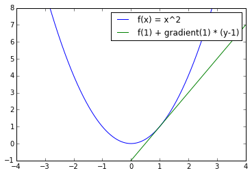
$f(y) = f(x) + \langle \nabla f(x), (y-x) \rangle + \frac{1}{2\eta}\norm{y-x}_{2}^2$

Note that $f(x) + \langle \nabla f(x), (y-x) \rangle$ is a linear approximation of $f$ , using the gradient at point $x$ . For example, take $f(x) = x^2$ , and let's approximate it at the point $x=1$ using its gradient:

Note as well that $\frac{1}{2\eta}\norm{y-x}_{2}^2$ is a term that penalizes points away from $x$ , with weight $\frac{1}{2\eta}$ , so that when $\eta$ gets smaller, we pay more to move away from the current point:

Summing the two terms, we have a quadratic approximation to the function at point $x$ :

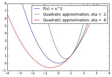
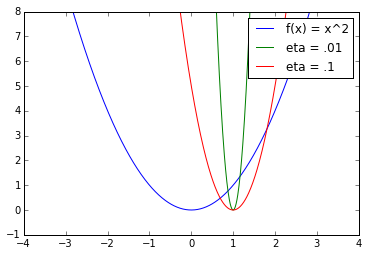
We will now show that gradient descent is in fact minimizing this quadratic approximation at each step. Before we do this, we can notice in the previous picture how important it is to get the right step size $\eta$ . In that case, if $\eta = .8$ , we will clearly go past the minimum of the function we are trying to optimize as we take one step from $x=1$ . Now, let's see what the minimum to the quadratic approximation is:

$\begin{align} min_y f(y) &= min_y \left\{ f(x) + \langle \nabla f(x), y-x \rangle + \frac{1}{2\eta}\norm{y - x}_2^2 \right\} \\ &= min_y \left\{ \langle \nabla f(x), y \rangle + \frac{1}{2\eta}\norm{y - x}_2^2 \right\} & \text{Removing terms that don't depend on y}\\ &= min_y \left\{ 2\eta \langle \nabla f(x), y \rangle + \norm{y - x}_2^2 \right\} & \text{Multiplying everything by $2\eta$}\\ &= min_y \left\{ 2\eta \langle \nabla f(x), y \rangle + \norm{y}_2^2 - 2\langle x,y \rangle + \cancel{\norm{x}^2_2} \right\} & \text{Expanding the square}\\ &= min_y \left\{ \norm{y - (x - \eta\nabla f(x))} \right\} & \text{Completing the square, ignoring irrelevant stuff} \end{align}$

It is easy to see that this function is minimized when $y = x - \eta\nabla f(x)$ , which is exactly the equation for the value of $x^{(k+1)}$ .

Convergence Analysis

We will prove a convergence bound for when the gradient of the function is Lipschitz continuous, i.e.:

$\norm{\nabla f(x) - \nabla f(y)}_2 \leq L \norm{x - y}_2 \quad(1)$

We already assumed that the function is convex and differentiable, i.e. $\forall y, x \in \mathbb{R}^n$ ,:

$f(y) \geq f(x) + \langle \nabla x, (y-x) \rangle \quad (2)$

First, we will prove that the following holds for any x,y:

$f(y) \leq f(x) + \langle \nabla f(x), y-x \rangle + \frac{L}{2} \norm{y-x}_2^2 \quad(3)$

Or equivalently:

$f(y) - f(x) -\langle \nabla f(x), y-x \rangle \leq \frac{L}{2} \norm{y-x}_2^2 \quad(4)$

To prove this, we will use an auxiliary function $g(t) = f(x + t(y - x))$ . Note that

$g(0) = f(x)$ $g(1) = f(y)$ $\nabla g(t) = \langle \nabla f(x + t(y-x)), y-x \rangle$ $\int_{0}^{1} \nabla g(t) dt = g(1) - g(0) = f(y) - f(x)$

We substitute the above to get :

$\begin{align} f(y) - f(x) -\langle \nabla f(x), y-x \rangle &= \int_{0}^{1} \langle \nabla f(x + t(y-x)), y-x \rangle dt - \langle \nabla f(x), y-x \rangle \\ &= \langle \int_{0}^{1} \nabla f(x + t(y-x)) dt - \nabla f(x), y-x \rangle \\ &\leq \int_{0}^{1} \norm{\nabla f(x + t(y-x)) - \nabla f(x)}_2 \norm{y-x}_2 & \text{by Cauchy–Schwarz} \\ &\leq \int_{0}^{1} L\norm{t(y-x)}_2\norm{y-x}_2 & \text{using (1) with $x + t(y-x)$ and $x$} \\ &= \int_{0}^{1} Lt\norm{(y-x)}_2^2\\ &= \frac{L}{2}\norm{y-x}_2^2 \end{align}$

Now we will use the above for iteration $x^{(k)}$ with $y = x^{(k+1)} = x^{(k)} - \eta \nabla f(x)$ . To simplify notation, let $x = x^{(k)}$ and $x^{+} = x^{(k+1)}$ .

$\begin{align} f(x^+) &\leq f(x) + \langle \nabla f(x), x - \eta \nabla f(x) - x \rangle + \frac{L}{2}\norm{x - \eta \nabla f(x) -x}_2^2 \\ &= f(x) + \langle \nabla f(x), -\eta \nabla f(x) \rangle + \frac{L}{2}\norm{ \eta \nabla f(x)}_2^2 \\ &= f(x) + -\eta \underbrace{\langle \nabla f(x), \nabla f(x) \rangle}_{\norm{\nabla f(x)}_2^2}+ \eta^2 \frac{L}{2}\norm{\nabla f(x)}_2^2 \\ &= f(x) -(1 - \frac{L\eta}{2}) \eta\norm{\nabla f(x)}_2^2 \\ \end{align}$

Now, take $\eta \leq \dfrac{1}{L}$ . This implies $1 - \dfrac{L\eta}{2} \leq 1 - \dfrac{1}{2} = \dfrac{1}{2}$ . Plugging this in the inequality above:

$f(x^+) \leq f(x) -\frac{\eta}{2}\norm{\nabla f(x)}_2^2 \quad (5)$

Note that we just proved that we are actually doing a descent - meaning that the function is decreasing (or staying the same) with each step we take, since $\eta > 0$ and $\norm{\nabla f(x)}_2^2 \geq 0$ .

Now we will use the convexity of $f(x)$ . Specifically, take $x^*$ to be the optimal solution to the problem. We can use the following linear approximation at $x^*$ (from the definition of convexity):

$f(x^*) \geq f(x) - \langle \nabla f(x), x - x^* \rangle$

Which equivalently is:

$f(x) \leq f(x^*) + \langle\nabla f(x), x - x^* \rangle$

Now that the inequality is in the right direction, we can directly plug it into (5):

$\begin{align} f(x^+) &\leq f(x^*) + \langle \nabla f(x), x - x^* \rangle -\frac{\eta}{2}\norm{\nabla f(x)}_2^2 \\ &= f(x^*) + \frac{1}{2 \eta}(2 \eta \langle \nabla f(x), x - x^* \rangle - \eta^2 \norm{\nabla f(x)}_2^2) \quad (6) \end{align}$

The reason we put $(6)$ in that particular form is because we will manipulate the term inside the parenthesis. Note the following:

$\begin{align} \norm{x - x^* - \eta \nabla f(x)}_2^2 = \norm{x - x^*}_2^2 -2 \eta \langle \nabla f(x), x - x^*\rangle + \eta^2 \norm{\nabla f(x)}_2^2 \end{align}$

Let the term inside the parenthesis of (6) be $Z$ . It is clear that $\norm{x - x^* - \eta \nabla f(x)}_2^2 = -Z + \norm{x - x^*}_2^2$ , and thus $Z = \norm{x - x^*}_2^2 - \norm{x - x^* - \eta \nabla f(x)}_2^2$ . From this, we get a modified form of (6):

$\begin{align} f(x^+) &\leq f(x^*) + \frac{1}{2 \eta}(\norm{x - x^*}_2^2 - \norm{\underbrace{x - \eta \nabla f(x)}_{x^+} - x^*}_2^2) \\ &= f(x^*) + \frac{1}{2 \eta}(\norm{x - x^*}_2^2 - \norm{x^+ - x^*}_2^2) \quad (6) \end{align}$

Now, all of this was just for a particular iteration. Now we will bound the sum over the difference between the $x$ of each iteration and the optimal $x^*$ :

$\begin{align} \sum_{i= 1}^k f(x^{(i)}) - f(x^{*}) &\leq \frac{1}{2 \eta}\sum_{i= 1}^k (\norm{x^{(i - 1)} - x^*}_2^2 - \norm{x^{(i)} - x^*}_2^2) & \text{We just applied (6)} \\ &= \frac{1}{2 \eta}\left(\norm{x^{(0)} - x^*}_2^2 - \cancel{\norm{x^{(1)} - x^*}_2^2} +\cancel{\norm{x^{(1)} - x^*}_2^2} - \norm{x^{(2)} - x^*}_2^2 \quad ... \right) & \text{Telescoping sum} \\ &= \frac{1}{2 \eta}(\norm{x^{(0)} - x^{*}}_2^2 - \norm{x^{(k)} - x^{*}}_2^2) \\ &\leq \frac{1}{2 \eta}(\norm{x^{(0)} - x^{*}}_2^2) \quad (7) \end{align}$

Now, all of this was just for a particular iteration. Now we will bound the sum over the difference between the $x$ of each iteration and the optimal $x^*$ :

This is our bound. Notice what it tells us: if the assumptions are met, and we use an appropriate constant stepsize, the distance between the loss at iteration $k$ and the optimum goes down at a rate that goes down at $O(\dfrac{1}{k})$ (linear in $k$ ), where the constant depends on how far our initial guess is from the optimal parameters.
What is an appropriate constant stepsize? Smaller than $\dfrac{1}{L}$ , meaning that we can take larger stepsizes if the Lipschitz constant of the gradients is small - which makes sense, because that would mean that the gradients can't be too big, which could cause us to overshoot.

We did a lot of steps, but notice the most important ones:

In (3), we bounded how much $f$ can change around any point $y$ , using the Lipschitz constant.
In (5), we showed that we are improving on the objective at each iteration, at a particular rate
From there, we just did math to see what happens after $k$ iterations

References

Written on April 3, 2015