Wed, Jan 05
Computing with parallel universes
Slides
|
- Course overview
- The experimental origins of quantum mechanics
- Quantum computing hype
-
Computational efficiency and computational models (deterministic, randomized, quantum) and contrasting behaviors for problems like integer multiplication, primality testing, and factorization
Relevant video lecture: ”\(10^{500}\) Parallel Universes”
|
| Basic structures of quantum computation |
Mon, Jan 10
Qubits
Lecture recording
Scribe notes
Suggested reading:
N&C 1.2-1.3, Mermin 1.1-1.2
|
Summary
-
Superpositions: Consider a system that can be in one of two states \(\ket{0}\) and \(\ket{1}\). Our first principle of quantum mechanics
says that if a quantum system can be in two basic states, then it can also be in any superposition of those states.
A superposition is of the form \(\alpha \ket{0} + \beta \ket{1}\) where \(\alpha\) and \(\beta\) are complex numbers and \(\abs{\alpha}^2 + \abs{\beta}^2 = 1\).
(Recall that if \(\alpha = a + bi\), then \(\abs{\alpha} = \sqrt{a^2 + b^2}\).)
A qubit is a unit vector in \(\begin{bmatrix} \alpha \\ \beta \end{bmatrix} \in \mathbb{C}^2\) that we think of as superposition \(\alpha \ket{0} + \beta \ket{1}\) of the
two basic states \(\ket{0}\) and \(\ket{1}\).
Here are some possible qubit states:
\[\qquad \ket{0},\ \ket{1},\ \tfrac{1}{\sqrt{2}}\ket{0} + \tfrac{1}{\sqrt{2}}\ket{1},\ 0.8 \ket{0} - 0.6 \ket{1},\ (\tfrac{1}{2} - \tfrac{i}{2}) \ket{0} - \tfrac{i}{\sqrt{2}} \ket{1}.\]
-
More generally, the state of \(d\)-dimensional quantum system is described by a unit vector
\(\begin{bmatrix} \alpha_1 \\ \alpha_2 \\ \vdots \\ \alpha_d \end{bmatrix} \in \mathbb{C}^d\) which we think of
as a superposition \(\alpha_1 \ket{1} + \alpha_2 \ket{2} + \cdots + \alpha_d \ket{d}\) of the basic states \(\ket{1},\ket{2},\ldots,\ket{d}\).
So we can think of \(\{\ket{1},\ket{2},\ldots,\ket{d}\}\) as the standard basis for \(\mathbb{C}^d\).
-
Bra-ket notation: In Dirac’s notation,
a vector of the form \(\ket{v}\) is a column vector, and \(\bra{v}\) is shorthand for the conjugate tranpose vector \(\ket{v}^*\).
One then writes the inner product of two vectors as
\[\ip{u}{v} \seteq \bar{u}_1 v_1 + \bar{u}_2 v_2 + \cdots + \bar{u}_d v_d,\]
where \(\overline{a+b i} = a - bi\) is the complex conjugate.
-
Measurements: Suppose we have a state \(\ket{\psi} \in \mathbb{C}^d\) and an orthonormal basis \(\ket{v_1},\ldots,\ket{v_d}\) of \(\C^d\).
We can express \(\ket{\psi}\) in this basis as
\[\ket{\psi} = \ip{v_1}{\psi} \,\ket{v_1} + \cdots + \ip{v_d}{\psi} \,\ket{v_d}.\]
Our second principle of quantum mechanics asserts
that when we measure \(\ket{\psi}\) in this basis, the state collapses to \(\ket{v_j}\) with probability \(|\ip{v_j}{\psi}|^2\).
Note that since \(\{\ket{v_1},\ldots,\ket{v_d}\}\) is an orthonormal basis, we have
\[|\ip{v_1}{\psi}|^2 + \cdots + |\ip{v_d}{\psi}|^2 = \ip{\psi}{\psi} = 1,\]
where the latter inequality follows since \(\ket{\psi}\) is a quantum state (and thus a unit vector).
Example:
Consider the orthornormal basis \(\{\ket{+},\ket{-}\}\) defined by
\[\begin{align*}
\ket{+} &\seteq \frac{1}{\sqrt{2}} \ket{0} + \frac{1}{\sqrt{2}} \ket{1} \\
\ket{-} &\seteq \frac{1}{\sqrt{2}} \ket{0} - \frac{1}{\sqrt{2}} \ket{1}.
\end{align*}\]
-
If we measure the state \(\ket{0}\) in this basis, we will obtain the state \(\ket{+}\) with
probability \(\ip{+}{0}^2 = 1/2\) and the state \(\ket{-}\) with probability \(|\ip{-}{0}|^2 = 1/2\).
-
If we measure the state \(\ket{\phi} = 0.8 \ket{0} - 0.6 \ket{1}\) in the \(\{\ket{+},\ket{-}\}\) basis, we will obtain the state
\(\ket{+}\) with probability
\[|\ip{+}{\phi}|^2 = \left(\frac{0.8}{\sqrt{2}} - \frac{0.6}{\sqrt{2}} \right)^2 = 0.02,\]
and we will obtain the state \(\ket{-}\) with probability
\[|\ip{-}{\phi}|^2 = \left(\frac{0.8}{\sqrt{2}} + \frac{0.6}{\sqrt{2}}\right)^2 = \frac{1.96}{2} = 0.98.\]
Related videos:
|
Wed, Jan 12
Single qubit transformations
Lecture recording
Scribe notes
Suggested reading:
N&C 1.3, Mermin 1.3
|
Summary
-
Our third principle of quantum mechanics is that one can perform any unitary operation on a qudit state \(\ket{\psi} \in \C^d\).
-
A unitary operation is a linear map that preserves the length of vectors.
Such maps can be described as \(d \times d\) complex matrices \(U\) with the property that \(U^* U = I\).
Equivalently, these are matrices \(U\) whose rows form an orthornomal basis of \(\C^d\) (equivalently,
whose columns form an orthonormal basis of \(\C^d\)).
-
As an example, for some angle \(\theta\), one can consider the rotation matrix
\[R_{\theta} = \begin{bmatrix} \cos \theta & - \sin \theta \\ \sin \theta & \cos \theta \end{bmatrix}\]
-
For instance, If we take \(\theta = 45^{\circ} = \frac{\pi}{4}\), then \(R_{45^{\circ}} \ket{0} = \ket{+}\) and
\(R_{45^{\circ}} \ket{1} = \frac{-1}{\sqrt{2}} \ket{0} + \frac{1}{\sqrt{2}} \ket{1}\).
-
Another unitary operation is the reflection
\[X \seteq \begin{bmatrix} 0 & 1 \\ 1 & 0 \end{bmatrix}\]
This is called “X” for historical reasons. It’s also known as the quantum NOT or the swap operator
since it satisfies \(X \ket{0} = \ket{1}\) and \(X \ket{1} = \ket{0}\).
-
You should check: If we want to change the basis \(\{\ket{0},\ket{1}\}\) into \(\{\ket{+},\ket{-}\}\), we can use the unitary operator \(X R_{45^{\circ}}\).
-
Since we can use unitary operations to map any orthonormal basis of \(\mathbb{C}^d\) to any other orthonormal basis,
we don’t need the ability to measure in an arbitrary basis \(\{\ket{u_1},\ldots,\ket{u_d}\}\).
If we let \(U\) be the matrix with \(\ket{u_1},\ldots,\ket{u_d}\) as the columns, then \(U^*\) satisfies
\(U^* \ket{u_j} = \ket{j}\), hence we can start with a state \(\ket{\psi}\), map it to \(U^* \ket{\psi}\),
measure in the standard basis \(\{\ket{1},\ldots,\ket{d}\}\), and then apply \(U\) to the collapsed state.
You should check: This is equivalent to measuring \(\ket{\psi}\) in the basis \(\{\ket{u_1},\ldots,\ket{u_d}\}\).
In other words, the outcome state is \(\ket{u_j}\) with probability \(|\ip{u_j}{\psi}|^2\).
-
In lecture, we saw how to use small rotations to implement the Elitzur-Vaidman quantum bomb detection algorithm.
Related videos:
|
Wed, Jan 19
Composite quantum systems
Suggested reading:
N&C 1.3; Mermin 1.4-1.6
|
Summary
-
We have seen that the quantum mechanical operations allowed on a quantum state \(\ket{\psi} \in \C^d\) are given by
the \(d \times d\) unitary matrices \(U \in \C^{d \times d}\).
-
In the case \(d=2\), examples of single-qubit gates include the real rotation matrices
\[R_{\theta} \seteq \begin{bmatrix} \cos \theta & -\sin \theta \\ -\sin \theta & \cos \theta \end{bmatrix},\]
the quantum NOT gate
\[X \seteq \begin{bmatrix} 0 & 1 \\ 1 & 0 \end{bmatrix},\]
and the Hadamard gate
\[H \seteq \frac{1}{\sqrt{2}} \begin{bmatrix} 1 & 1 \\ 1 & -1 \end{bmatrix}.\]
-
We can encode a two-qubit state as a vector \(\ket{\psi} \in \C^4\) using the basis
\[\{ \ket{00}, \ket{01}, \ket{10}, \ket{11} \} =
\left\{ \begin{bmatrix} 1 \\ 0 \\ 0 \\ 0 \end{bmatrix},
\begin{bmatrix} 0 \\ 1 \\ 0 \\ 0 \end{bmatrix},
\begin{bmatrix} 0 \\ 0 \\ 1 \\ 0 \end{bmatrix},
\begin{bmatrix} 0 \\ 0 \\ 0 \\ 1 \end{bmatrix} \right\}\]
-
Let us consider three different ways of representing the \(2\)-qubit controlled NOT gate \(\mathsf{CNOT}\):
-
We can write it as the matrix
\[\mathsf{CNOT} =
\begin{bmatrix}
1 & 0 & 0 & 0 \\
0 & 1 & 0 & 0 \\
0 & 0 & 0 & 1 \\
0 & 0 & 1 & 0
\end{bmatrix}\]
-
Equivalently, we can express its action on an orthornormal basis:
\[\begin{align*}
\ket{00} & \to \ket{00} \\
\ket{01} & \to \ket{01} \\
\ket{10} & \to \ket{11} \\
\ket{11} & \to \ket{10}.
\end{align*}\]
The first bit is the control bit, and it is simply copied to the output.
If the first bit is \(0\), we leave the second bit unchanged.
But if the first is \(1\), we perform a NOT on the second bit.
-
Finally, we can write it in the quantum circuit notation:
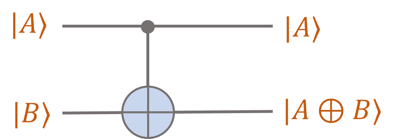
Note the suggestive notation: The first bit is passed through unchanged, while the second bit
becomes the XOR of the first two bits.
-
Another \(2\)-qubit gate is the swap gate:
\[\mathsf{SWAP} =
\begin{bmatrix}
1 & 0 & 0 & 0 \\
0 & 0 & 1 & 0 \\
0 & 1 & 0 & 0 \\
0 & 0 & 0 & 1
\end{bmatrix}\]
As the name suggests, this swaps the first and second qubits:
\[\begin{align*}
\ket{00} & \to \ket{00} \\
\ket{01} & \to \ket{10} \\
\ket{10} & \to \ket{01} \\
\ket{11} & \to \ket{11}.
\end{align*}\]
-
If we have two qubits \(\ket{\psi},\ket{\phi} \in \C^2\) and we want to apply a \(\mathsf{CNOT}\) gate to them, we
need a way of representing the composite state \(\ket{\psi} \ket{\phi}\) as a vector in \(\C^4\).
This will be the tensor product \(\ket{\psi} \otimes \ket{\phi}\).
Our fourth principle of quantum mechanics asserts that
if \(\ket{\psi} \in \C^m\) and \(\ket{\phi} \in \C^n\) are two quantum states, then their joint quantum system is described
by the state \(\ket{\psi} \otimes \ket{\phi} \in \C^{mn}\). Recall that the tensor product of two vectors \(\vec{u} \in \C^m\)
and \(\vec{v} \in \C^n\) is the vector \(\vec{u} \otimes \vec{v} \in \C^{m \times n}\) given by \((\vec{u} \otimes \vec{v})_{ij} = u_i v_j\).
-
Examples:
\[\begin{align*}
\ket{0} \otimes \ket{+} &= \ket{0} \otimes \left(\frac{1}{\sqrt{2}} \ket{0} + \frac{1}{\sqrt{2}} \ket{1}\right)
= \frac{1}{\sqrt{2}} \ket{0} \otimes \ket{0} + \frac{1}{\sqrt{2}} \ket{0} \otimes \ket{1}
= \frac{1}{\sqrt{2}} \ket{00} + \frac{1}{\sqrt{2}} \ket{01} \\
\ket{+} \otimes \ket{0} &= \left(\frac{1}{\sqrt{2}} \ket{0} + \frac{1}{\sqrt{2}} \ket{1}\right) \otimes \ket{0}
= \frac{1}{\sqrt{2}} \ket{0} \otimes \ket{0} + \frac{1}{\sqrt{2}} \ket{1} \otimes \ket{0}
= \frac{1}{\sqrt{2}} \ket{00} + \frac{1}{\sqrt{2}} \ket{10}.
\end{align*}\]
Note that we have used the shorthand \(\ket{0} \otimes \ket{0} = \ket{00}, \ket{0} \otimes \ket{1} = \ket{01}\), etc.
We have also used bilinearity of the tensor product:
\[\begin{align*}
(a+a') \otimes b &= a \otimes b + a' \otimes b \\
a \otimes (b+b') &= a \otimes b + a \otimes b' \\
(\lambda a) \otimes b &= \lambda (a \otimes b) = a \otimes (\lambda b), \quad \forall \lambda \in \C.
\end{align*}\]
-
This allows us to evaluate arbitrary quantum circuits. For instance, consider:
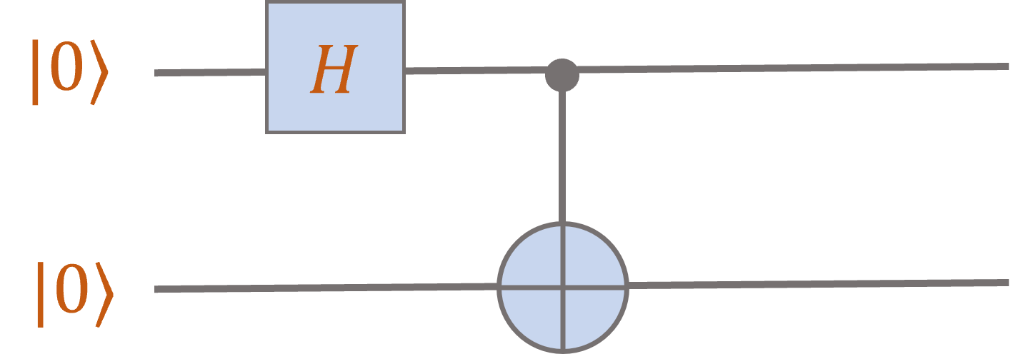
Applying a Hadamard gate to the first qubit yields \(H \ket{0} = \ket{+} = \frac{1}{\sqrt{2}} \ket{0} + \frac{1}{\sqrt{2}} \ket{1}\).
The tensor product rule tells us that the joint state of the two qubits after the Hadamard gate is given by
\[\ket{+} \otimes \ket{0} = \frac{1}{\sqrt{2}} \ket{00} + \frac{1}{\sqrt{2}} \ket{10}.\]
Now we can apply the \(\mathsf{CNOT}\) gate. By linearity, we can consider its action on each piece \(\ket{00} \mapsto \ket{00}\) and \(\ket{10} \mapsto \ket{11}\), hence
the output of the circuit is the state
\[\ket{\mathrm{bell}} = \frac{1}{\sqrt{2}} \ket{00} + \frac{1}{\sqrt{2}} \ket{11}.\]
-
This is called the Bell state. Its importance lies in the fact that it’s entangled, i.e., there is
now way to write \(\ket{\mathrm{bell}} = \ket{\psi} \otimes \ket{\phi}\) for single qubit states
\(\ket{\psi},\ket{\phi} \in \C^2\).
Indeed, suppose we could write \(\frac{1}{\sqrt{2}} \begin{bmatrix} 1 \\ 0 \\ 0 \\ 1 \end{bmatrix} = \ket{\mathrm{bell}} = \begin{bmatrix} a_0 \\ a_1 \end{bmatrix} \otimes
\begin{bmatrix} b_0 \\ b_1 \end{bmatrix} = \begin{bmatrix} a_0 b_0 \\ a_0 b_1 \\ a_1 b_0 \\ a_1 b_1 \end{bmatrix}\).
Notice that the product of the first and last entries of the latter vector is \(a_0 b_0 a_1 b_1\), and this is also equal
to the product of the two middle entries. Since that property doesn’t hold for \(\ket{\mathrm{bell}}\), no such
decomposition is possible.
A composite state that cannot be written as a tensor product of joint states is said to be entangled.
-
Let’s try one more: (You should verify the calculations!)
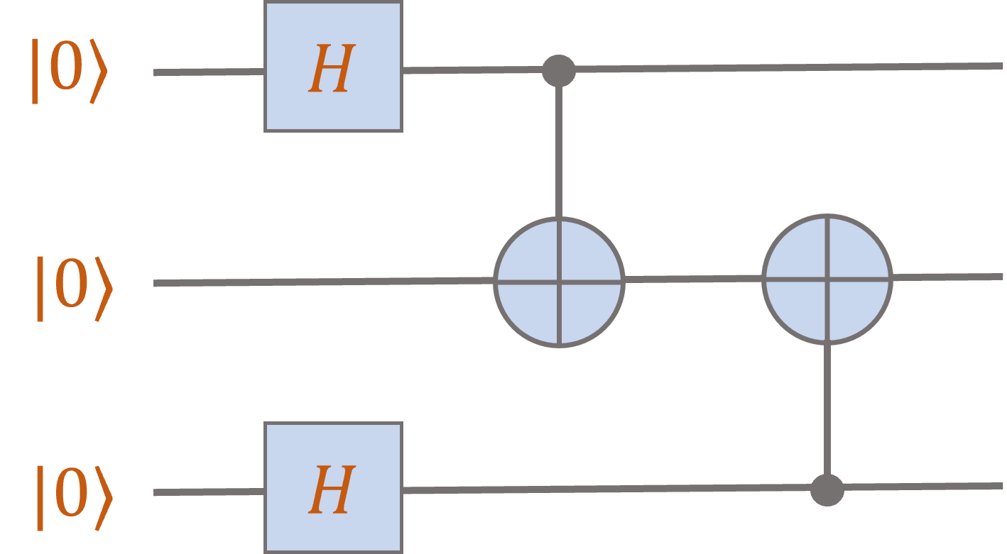
After the first two Hadamard gates, the system is in the state
\[\ket{+} \otimes \ket{0} \otimes \ket{+} = \frac{1}{\sqrt{2}} \ket{00} \otimes \ket{+} + \frac{1}{\sqrt{2}} \ket{10} \otimes \ket{+}.\]
Now applying the first controlled-NOT gate to the first two qubits yields the state
\[\frac{1}{\sqrt{2}} \ket{00} \otimes \ket{+} + \frac{1}{\sqrt{2}} \ket{11} \otimes \ket{+}
= \frac{1}{2} \ket{000} + \frac{1}{2} \ket{001} + \frac{1}{2} \ket{110} + \frac{1}{2} \ket{111}.\]
Finally, applying the second controlled-NOT bit to the second two qubits yields the state
\[\frac{1}{2} \ket{000} + \frac{1}{2} \ket{011} + \frac{1}{2} \ket{110} + \frac{1}{2} \ket{101}.\]
-
Recall that \(\mathsf{NOT}\) and 2-bit \(\mathsf{AND}\) gates are universal for classical computation (Problem 1 on HW1),
and \(\mathsf{NOT}\), 2-bit \(\mathsf{AND}\), and \(\mathsf{FLIP}(1/3)\) gates are universal for randomized computation (Problem 2 on HW1).
Here’s a very useful fact: Single qubit gates and the 2-qubit \(\mathsf{CNOT}\) gate are universal for quantum computation,
in the sense that every unitary \(U \in \mathbb{C}^{2^d \times 2^d}\) can be approximated arbitrarily well by a circuit on
\(d\) input qubits consisting
only of such gates. (Note: This doesn’t tell us anything about the size of such a circuit!)
Related videos:
|
Mon, Jan 24
Operations on subsystems and partial measurements
Suggested reading:
N&C 2.2, Mermin 1.7-1.12
|
Summary
-
Tensor products:
-
Note that the defining characteristic of the tensor product is multilinearity, which simply means
that for vectors \(v_1 \in \C^{n_1}, v_2 \in \C^{n_2}, \ldots, v_k \in \C^{n_k}\), the expression
\[v_1 \otimes v_2 \otimes \cdots \otimes v_k\]
is linear in each vector \(v_i\) so that, for instance,
\[v_1 \otimes (u_2 + v_2) \otimes \cdots \otimes v_k = v_1 \otimes u_2 \otimes \cdots \otimes v_k + v_1 \otimes v_2 \otimes \cdots \otimes v_k.\]
Note that this is just like how normal multiplication distributes over addition. But do note that tensor products are definitely
not commutative: The vectors \(v_1 \otimes v_2\) and \(v_2 \otimes v_1\) are not equal unless \(v_1 = v_2\).
-
Given matrices \(A_1 \in \C^{m_1 \times n_1}, A_2 \in \C^{m_2 \times n_2}, \cdots, A_k \in \C^{m_k \times n_k}\), we can form
the tensor product
\[A_1 \otimes A_2 \otimes \cdots \otimes A_k\]
One can think of this object in various way, e.g., we can meaningfully write
\[(A_1 \otimes A_2 \otimes \cdots \otimes A_k)_{i_1 j_1, i_2 j_2, \ldots, i_k j_k} = (A_1)_{i_1 j_1} (A_2)_{i_2 j_2} \cdots (A_k)_{i_k j_k},\]
thinking of this as a multidimensional array of \(m_1 \cdot n_1 \cdot m_2 \cdot n_2 \cdots m_k \cdot n_k\) numbers.
It is most useful to think of it as a linear map taking vectors in \(\C^{n_1} \otimes \C^{n_2} \otimes \cdots \otimes \C^{n_k}\)
to vectors in \(\C^{m_1} \otimes \C^{m_2} \otimes \cdots \otimes \C^{m_k}\), where the map is applied just as you would expect:
\[(A_1 \otimes A_2 \otimes \cdots \otimes A_k) (v_1 \otimes v_2 \otimes \cdots \otimes v_k)
=A_1 v_1 \otimes A_2 v_2 \otimes \cdots \otimes A_k v_k.\]
-
Unitaries acting on subsystems: Recall this quantum circuit from the previous lecture.
Just before the last \(\mathsf{CNOT}\) gate, the 3-qubit state is
\[\frac{1}{\sqrt{2}} \ket{00} \otimes \ket{+} + \frac{1}{\sqrt{2}} \ket{11} \otimes \ket{+}
= \frac{1}{2} \ket{000} + \frac{1}{2} \ket{001} + \frac{1}{2} \ket{110} + \frac{1}{2} \ket{111}.\]
The last \(\mathsf{CNOT}\) gate acts only on the last two qubits, but we need to define its action
on a 3-qubit state. Our fifth principle of quantum mechanics tells us how to
applying a unitary to a subsystem affects the entire state.
Note that, by linearity, we need only understand its action on each of the basis states \(\ket{000}\), \(\ket{001}\), \(\ket{110}\), and \(\ket{111}\).
Recall that \(\ket{001} = \ket{0} \otimes \ket{01}\). The fifth princple says that to apply the \(\mathsf{CNOT}\) gate to the last two bits,
we just act in that component of the tensor product:
\[\ket{0} \otimes \ket{01} \mapsto \ket{0} \otimes \mathsf{CNOT} \ket{01} = \ket{0} \otimes \ket{11}.\]
Equivalently, in order to apply \(\mathsf{CNOT}\) to the last two qubits, we apply the matrix
\(I \otimes \mathsf{CNOT}\) to the entire 3-qubit state, where \(I\) is the identity matrix on the first qubit.
Thus this circuit outputs the state
\[\frac{1}{2} \ket{000} + \frac{1}{2} \ket{011} + \frac{1}{2} \ket{110} + \frac{1}{2} \ket{101}.\]
-
Note that there is no reason that the \(\mathsf{CNOT}\) needs to act on “adjacent” qubits (adjacency here is just an artifact
of how we drew the circuits). We could equally well consider a circuit where the final \(\mathsf{CNOT}\) gate acts on
the first and third qubits:
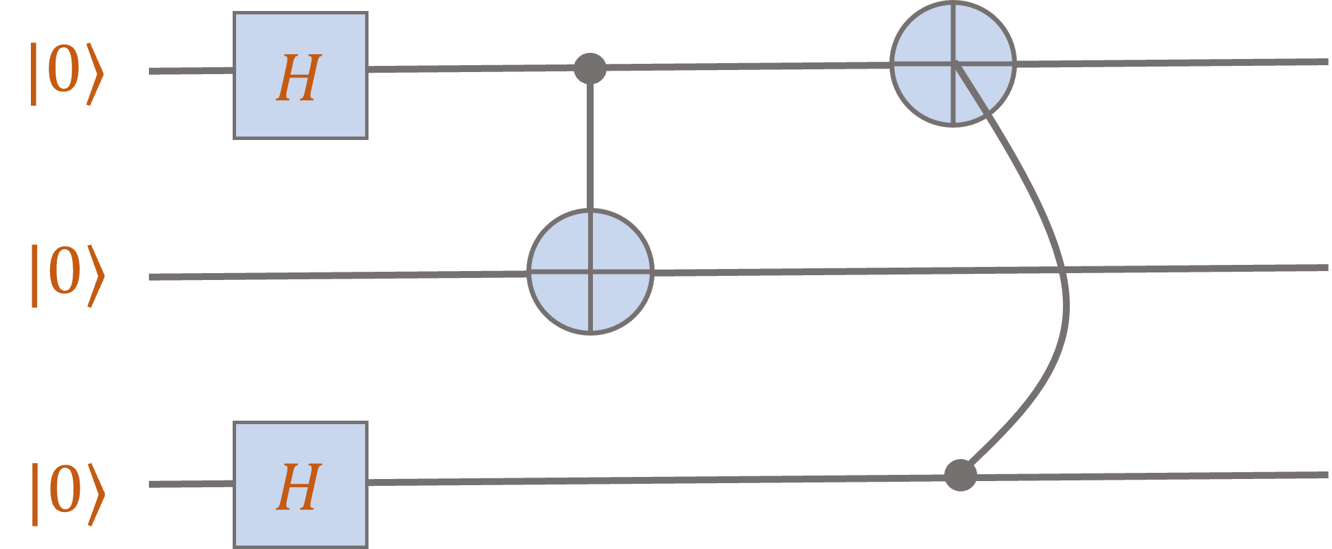
You should check that the output state is
\[\frac12 \ket{000} + \frac12 \ket{101} + \frac12 \ket{110} + \frac12 \ket{011}.\]
It is a coincidence that these two circuits give the same output on input \(\ket{000}\).
(It is not true that they give the same output for every input.)
-
Partial measurements:
Suppose that we have a 2-qubit state
\[\alpha_{00} \ket{00} + \alpha_{01} \ket{01} + \alpha_{10} \ket{10} + \alpha_{11} \ket{11}.\]
Suppose also that Alice takes the first qubit, Bob takes the second, and then Alice
measures her qubit in the \(\{\ket{0},\ket{1}\}\) basis. The new joint state is given by the Born rule,
which agrees with the standard notion of conditional probabilities.
With probability \(p_0 \seteq |\alpha_{00}|^2 + |\alpha_{01}|^2\), Alice measures outcome “0” and
the joint state collapses to
\[\frac{\alpha_{00}}{\sqrt{p_0}} \ket{00} + \frac{\alpha_{01}}{\sqrt{p_0}} \ket{01}
= \ket{0} \otimes \left(\frac{\alpha_{00}}{\sqrt{p_0}} \ket{0} + \frac{\alpha_{01}}{\sqrt{p_0}} \ket{1}\right),\]
and with probability \(p_1 \seteq |\alpha_{10}|^2 + \alpha_{11}|^2\), Alice measures outcome “1”
and the joint state collapses to
\[\frac{\alpha_{10}}{\sqrt{p_1}} \ket{10} + \frac{\alpha_{11}}{\sqrt{p_1}} \ket{11}
= \ket{1} \otimes \left(\frac{\alpha_{10}}{\sqrt{p_1}} \ket{0} + \frac{\alpha_{11}}{\sqrt{p_1}} \ket{1}\right),\]
Related videos:
|
| Basics of quantum information |
Wed, Jan 26
Bell's theorem and the EPR paradox
Suggested reading:
N&C 2.6
|
Summary
-
The CHSH game can be described as follows:
There are three participants: Alice, Bob, and a Referee. The Referee chooses
two uniformly random bits \(x,y \in \{0,1\}\) and sends \(x\) to Alice and \(y\) to Bob.
Alice outputs a bit \(A(x)\) and Bob outputs a bit \(B(y)\), and their goal is to achieve the outcome
\[\begin{equation}\label{eq:goal}
A(x) \oplus B(y) = x \wedge y.
\end{equation}\]
It is easy to check that for any of the 16 pairs of strategies for Alice and Bob,
described by functions \(A,B : \{0,1\} \to \{0,1\}\), there must be at least one choice
\(x,y \in \{0,1\}\) that fails to achieve the goal \eqref{eq:goal}.
Thus the maximum success probability for Alice and Bob is at most \(3/4 = 75\%\).
-
Even if Alice and Bob have shared random bits, they cannot achieve better than \(75\%\).
Indeed, let \(\mathbf{r} = r_1 r_2 \ldots r_m\) be a string of random bits, then
for every fixed choice of \(r\), we have
\(\mathbb{P}_{x,y}[A_r(x) = B_r(y)] \leq 3/4.\)
So this still holds whene we average over the random string \(\mathbf{r}\).
-
It turns out that if Alice and Bob share an EPR pair \(\ket{\psi} = \frac{1}{\sqrt{2}} (\ket{00}+\ket{11})\),
then they can do strictly better than just by using shared randomness: They can achieve success probability
\[\left(\cos \frac{\pi}{8}\right)^2 = \frac{1}{2} + \frac{1}{2\sqrt{2}} \approx 0.853\cdots.\]
-
The protocol is as follows:
-
Alice:
-
\(x=0\):
Alice measures her qubit in the \(\{\ket{0},\ket{1}\}\) basis and outputs
a bit according to her measurement:
\[\begin{align*}
\ket{0} &\mapsto A = 0\,, \\
\ket{1} &\mapsto A = 1\,.
\end{align*}\]
-
\(x=1\):
Alice measures her qubit in the \(\{\ket{+},\ket{-}\}\) basis and outputs
a bit according to her measurement:
\[\begin{align*}
\ket{+} \mapsto A = 0\,, \\
\ket{-} \mapsto A = 1\,.
\end{align*}\]
-
Bob:
-
\(y=0\):
Bob measures his qubit in the basis \(\{\ket{a_0},\ket{a_1}\}\) and outputs \(B=0\) or \(B=1\), respectively.
\[\begin{align*}
\ket{a_0} &= \left(\cos \frac{\pi}{8}\right) \ket{0} + \left(\sin \frac{\pi}{8}\right) \ket{1}\,, \\
\ket{a_1} &=\left(-\sin \frac{\pi}{8}\right) \ket{0} + \left(\cos \frac{\pi}{8}\right) \ket{1}\,.
\end{align*}\]
Equivalently, this is the standard basis rotated by \(\pi/8\).
-
\(y=1\):
Bob measures his qubit in the basis \(\{\ket{b_0},\ket{b_1}\}\) and outputs \(B=0\) or \(B=1\), respectively.
\[\begin{align*}
\ket{b_0} &= \left(\cos \frac{\pi}{8}\right) \ket{0} - \left(\sin \frac{\pi}{8}\right) \ket{1}\,, \\
\ket{b_1} &=\left(\sin \frac{\pi}{8}\right) \ket{0} + \left(\cos \frac{\pi}{8}\right) \ket{1}\,.
\end{align*}\]
Equivalently, this is the standard basis rotated by \(-\pi/8\).
-
For example, let’s analyze the success
probability in the case \(x=y=0\). Since \(x \wedge y = 0\), we need \(A \neq B\), i.e.,
we need the measurement outcomes \(\ket{0},\ket{a_0}\) or \(\ket{1},\ket{a_1}\).
With probability \(1/2\), Alice measures \(\ket{0}\) and Bob’s qubit collapses to the state \(\ket{0}\).
Then the probability he measures \(\ket{a_0}\) is \(|\ip{a_0}{0}|^2 = (\cos \frac{\pi}{8})^2\).
With probability \(1/2\), Alice measures \(\ket{1}\) and Bob’s qubit collapses to the state \(\ket{1}\).
Then the probability he measures \(\ket{a_1}\) is \(|\ip{a_1}{1}|^2 = (\cos \frac{\pi}{8})^2\).
Hence the overall success probability is \((\cos \frac{\pi}{8})^2\).
-
As an exercise, you should try repeating the analysis from lecture for the other three cases.
For the case where \(x=1\), it helps to verify first that the EPR pair can equivalently be written as
\[\ket{\psi} = \frac{1}{\sqrt{2}} \left(\ket{++} + \ket{--}\right).\]
-
In the early 1980s, experiments acheived \(84\%\).
-
In 2014, it was verified at large scales (1.3km).
-
The famous Tsirelson inequality shows that no
quantum strategy can do better than \((\cos \frac{\pi}{8})^2\).
-
Some philosophical discussion around the EPR paradox and Bell’s theorem
Related videos:
|
Mon, Jan 31
The No-Cloning Theorem and quantum teleportation
Suggested reading:
N&C 12.1 & 1.3.7; Mermin 2.1 & 6.5
|
Summary
-
No-cloning Theorem: There is no quantum operation that starts with a state \(\ket{\psi}\) and outputs two copies \(\ket{\psi} \otimes \ket{\psi}\).
More formally, there is no quantum circuit that takes as input a qubit \(\ket{\psi} = \alpha \ket{0} + \beta \ket{1}\)
along with ancilliary bits \(\ket{0000\cdots 0}\) and outputs a state \(\ket{\psi} \otimes \ket{\psi} \otimes \ket{\mathrm{garbage}}\)
where the first two qubits are copies of \(\ket{\psi}\).
Note that a \(\mathsf{CNOT}\) successfully copies the control bits \(\ket{0}\) and \(\ket{1}\) when the other input is \(\ket{0}\):
\[\begin{align*}
\mathsf{CNOT} \ket{0} \ket{0} &= \ket{0} \ket{0}\,, \\
\mathsf{CNOT} \ket{1} \ket{0} &= \ket{1} \ket{1}\,.
\end{align*}\]
On the other hand, \(\mathsf{CNOT}\) fails to copy \(\ket{+}\):
\[\mathsf{CNOT} \ket{+} \ket{0} = \frac{1}{\sqrt{2}} \left(\ket{00} + \ket{11}\right).\]
As we know, this is not a tensor product state. To successfully clone, we wanted to get the state
\[\ket{+}\ket{+} = \frac12 \left(\ket{00}+\ket{01}+\ket{10}+\ket{11}\right).\]
-
Proof of the No-Cloning Theorem:
Suppose we have a quantum circuit without intermediate measurements that clones an input qubit. (We will see later in the course that
measurements can always be deferred to the end of a quantum computation. This is called the
Principle of Deferred Measurement.)
Consider its operation on \(\ket{0}\),\(\ket{1}\), and \(\ket{+}\):
\[\begin{align}
\ket{0} \ket{00\cdots0} &\mapsto \ket{0} \ket{0} \otimes \ket{f(0)} \label{eq:f0} \\
\ket{1} \ket{00\cdots0} &\mapsto \ket{1} \ket{1} \otimes \ket{f(1)} \label{eq:f1} \\
\ket{+} \ket{00\cdots0} &\mapsto \ket{+} \ket{+} \otimes \ket{f(+)}\,, \label{eq:f2} \\
\end{align}\]
where \(f(0),f(1),f(+)\) are some arbitrary states depending on the input. Then since the circuit must correspond
to multiplication by a unitary matrix, it must act linearly, and by \(\eqref{eq:f0}\) and \(\eqref{eq:f1}\), its output on \(\ket{+} \ket{00\cdots0} = \left(\frac{1}{\sqrt{2}} \ket{0}+ \frac{1}{\sqrt{2}} \ket{1}\right)\ket{00\cdots0}\) must be equal to
\[\frac{1}{\sqrt{2}} \left(\ket{0} \ket{0} \ket{f(0)} + \ket{1} \ket{1} \ket{f(1)}\right).\]
But this can never be equal to the RHS of \(\eqref{eq:f2}\) since
\[\ket{+} \ket{+} \otimes \ket{f(+)} = \frac{1}{2} \left(\ket{00}+\ket{01}+\ket{10}+\ket{11} \right) \ket{f(+)}.\]
(Two see that these two states cannot be equal, considering measuring the first two qubits.)
-
The No-Cloning Theorem implies that it is impossible to learn the amplitudes of a qubit \(\ket{\psi} = \alpha \ket{0} + \beta \ket{1}\) since
if we knew \(\alpha\) and \(\beta\), we could build a circuit that, on input \(\ket{0}\), would output \(\ket{\psi}\).
And then we could make as many copies of \(\ket{\psi}\) as we wanted. Just for review, note that the following
single qubit unitary gate maps \(\ket{0}\) to \(\ket{\psi}\):
\[\begin{bmatrix}
\alpha & -\beta \\ \beta & \alpha
\end{bmatrix}
\ket{0} = \alpha \ket{0} + \beta\ket{1}.\]
-
Quantum tomography studies the best way to learn a quantum state \(\ket{\psi}\)
given many copies \(\ket{\psi} \otimes \ket{\psi} \otimes \cdots \otimes \ket{\psi}\).
-
Quantum teleportation: This is the idea that if Alice and Bob share an EPR pair \(\ket{\mathrm{bell}} = \frac{1}{\sqrt{2}} (\ket{00}+\ket{11})\),
then Alice can “teleport” an arbitrary qubit state to Bob by sending him only two bits of classical information.
Here is a sketch: Alice has the qubit state \(\ket{\psi} = \alpha \ket{0} + \beta \ket{1}\) and the first qubit of the EPR pair \(\ket{\mathrm{bell}}\),
and Bob has the second qubit of \(\ket{\mathrm{bell}}\).
Alice first applies a \(\mathsf{CNOT}\) gate to her two qubits and the state evolves as
\[(\alpha \ket{0} + \beta \ket{1}) \frac{1}{\sqrt{2}} \left(\ket{00}+\ket{11}\right) \mapsto
\frac{\alpha}{\sqrt{2}} \ket{0} \left(\ket{00} + \ket{11}\right) +
\frac{\beta}{\sqrt{2}} \ket{1} \left(\ket{10} + \ket{01}\right)\]
She then applies a Hadamard gate to her first qubit, giving the state
\[\begin{align*}
\frac{1}{2} \ket{00} &\left(\alpha \ket{0} + \beta \ket{1}\right) + \\
\frac{1}{2} \ket{01} &\left(\beta \ket{0} + \alpha \ket{1}\right) + \\
\frac{1}{2} \ket{10} &\left(\alpha \ket{0} - \beta \ket{1}\right) + \\
\frac{1}{2} \ket{11} &\left(-\beta \ket{0} + \alpha \ket{1}\right)\,.\\
\end{align*}\]
Alice now measures her two qubits, giving each of the four outcomes \(\{00,01,10,11\}\) with probability \(1/2\).
Bob’s state collapses to one of the four options above, and when he receives the message from Alice,
it tells him which unitary he can apply to convert his state to \(\alpha \ket{0} + \beta \ket{1}\)!
For example, if the messages is \(00\), he just applies the identity. If the message is \(01\), he applies the unitary
\(\begin{bmatrix} 0 & 1 \\ 1 & 0 \end{bmatrix}\), etc.
Related videos:
|
Wed, Feb 02
Quantum coins and one-time pads
|
Summary
-
A scheme for quantum money: The No-Cloning Theorem suggests that we might be able to achieve true “copy protection”
using properties of quantum states. As an example, we can try to design a scheme for making “coins” that can
be verified as real, but not copied.
-
In class we studied the Wiesner scheme, where the bank chooses uniformly at random
a serial number \(s \in \{0,1\}^n\) and a string \(q \in \{0,1,+,-\}^n\) and constructs the state
\[\ket{\psi} = \ket{q_1} \ket{q_2} \cdots \ket{q_n}.\]
The coin is then the pair \((s,\ket{\psi})\).
-
The bank verifies the coin by measuring every qubit of \(\psi\) in either the \(\{\ket{0},\ket{1}\}\) basis (for \(q_i \in \{0,1\}\)) or
the \(\{\ket{+},\ket{-}\}\) basis (for \(q_i \in \{+,-\}\)) and checking that the answer is equal to \(q_i\).
(See Homework #3.)
-
We saw that in this scheme, the bank should not return coins that have been verified as valid, since otherwise there
is a clever attack to learn the state \(\ket{\psi}\). The attack is similar to detecting the Elitzur-Vaidman bomb.
Let \(R_{\varepsilon} = \begin{bmatrix} \cos(\varepsilon) & \sin(\varepsilon) \\ -\sin(\varepsilon) & \cos(\varepsilon) \end{bmatrix}\) be a rotation by angle \(\varepsilon\).
Choose a sufficiently large even number \(k\) and take \(\varepsilon = \frac{\pi}{2k}\).
The attacker tries to learn each qubit of \(\ket{\psi}\) in succession. Consider \(\ket{q_1}\). The attacker introduces an auxiliary qubit
that starts in the \(\ket{0}\) state, so the system is \(\ket{0} \ket{q_1}\).
Then the attacker repeats the following \(k\) times:
-
Apply \(R_{\varepsilon}\) to the first qubit, and a \(\mathsf{CNOT}\) gate to the pair, where the first bit is the control bit.
-
Ask the bank to verify \(\ket{\psi}\).
-
Consider the the four cases:
-
If \(\ket{q_1} = \ket{0}\), a single round yields the state
\[\cos(\varepsilon) \ket{00} + \sin(\varepsilon) \ket{11}.\]
When the bank measures the second qubit in the \(\{\ket{0},\ket{1}\}\) basis,
it detects fraud with probility \(\sin(\varepsilon)^2 \leq \varepsilon^2\) (for \(\varepsilon\) small),
and otherwise measures \(\ket{0}\) and the state collapses to the initial state \(\ket{00}\).
If fraud is not detected for \(k\) rounds, the resulting state is \(\ket{00}\).
-
If \(\ket{q_1} = \ket{1}\), a single round yields the state
\[\cos(\varepsilon) \ket{01} + \sin(\varepsilon) \ket{10}.\]
When the bank measures the second qubit in the \(\{\ket{0},\ket{1}\}\) basis,
it detects fraud with probility \(\sin(\varepsilon)^2 \leq \varepsilon^2\) (for \(\varepsilon\) small),
and otherwise measures \(\ket{1}\) and the state collapses to the initial state \(\ket{01}\).
If fraud is not detected for \(k\) rounds, the resulting state is \(\ket{01}\).
-
If \(\ket{q_1} = \ket{-}\), a single round yields the state
\[\cos(\varepsilon) \ket{0,-} - \sin(\varepsilon) \ket{1,-}.\]
When the bank measures the second qubit in the \(\{\ket{+},\ket{-}\}\) basis,
it always gets the correct outcome \(\ket{+}\), and the state collapses to \(R_{-\varepsilon} \ket{0} \ket{-}\).
In the next round, we first apply \(R_{\varepsilon}\), yielding \(\ket{0} \ket{-}\). The bank measures
the second qubit correctly, and the state collapses to \(\ket{0} \ket{-}\).
Therefore after \(k\) rounds (recall that \(k\) is even!), the resulting state is \(\ket{0} \ket{+}\).
-
If \(\ket{q_1} = \ket{+}\), a single round yields the state
\[\cos(\varepsilon) \ket{0,+} + \sin(\varepsilon) \ket{1,+}.\]
When the bank measures the second qubit in the \(\{\ket{+},\ket{-}\}\) basis,
it always gets the correct outcome \(\ket{+}\), and the state collapses to \(R_{\varepsilon} \ket{0} \ket{+}\).
After \(k\) rounds, we have applied a rotation by \(k \cdot \varepsilon = \frac{\pi}{2}\), hence the resulting state is \(\ket{1} \ket{+}\).
-
If we are not caught cheating, then after all \(k\) rounds, we can measure the first bit in the \(\{\ket{0},\ket{1}\}\) basis
and with certainty determine whether \(q_1 = +\) or \(q_1 \neq +\).
Our chance of being caught is at most \(\varepsilon^2 k = \frac{1}{k} \left(\frac{\pi}{2}\right)^2\).
By slighty modifying the protocol (exercise: what’s the modification?), we can also test whether \(q_1 = -\).
If neither of these is true, we know that we can measure \(\ket{q_1}\) in the \(\{\ket{0},\ket{1}\}\) and determine
its value with certainty.
So we can determine \(q_1\) with a probability of at most \(2 \varepsilon^2 k = \frac{1}{k} \frac{\pi^2}{2}\) of getting caught.
Now repeat this for every qubit \(\ket{q_i}\). We determine all the values with at most a \(\frac{n}{k} \frac{\pi^2}{2}\) chance of getting caught.
So by setting \(k = 1000 n\) (say), we can successfully learn \(\ket{\psi}\) with less than a half percent chance we are caught.
(And then we can make as many copies of \((s,\ket{\psi})\) as we like!)
Related videos:
|
| Quantum algorithms |
Mon, Feb 07
Bernstein-Vazirani
Suggested reading:
Mermin 2.1-2.4
|
Summary
-
Definition: If \(F : \{0,1\}^n \to \{0,1\}^m\) is a function from \(n\) bits to \(m\) bits, then a quantum circuit \(Q_F\)
implementing \(F\) is one that maps
\[\begin{equation}\label{eq:standard}
Q_F : \ket{x} \ket{y} \ket{00\cdots 0} \mapsto \ket{x} \ket{y \oplus F(x)} \ket{00\cdots 0},
\end{equation}\]
Here, \(\oplus\) represents the bitwise exclusive-or operation.
The first register is on \(n\) qubits, and the third register is on \(m\) qubits.
The additional \(0\) qubits are called ancillas.
The size of the circuit is the number of basic quantum gates.
-
If \(F : \{0,1\}^n \to \{0,1\}^m\) is computed by a classical circuit with \(g\) gates, then there is a quantum
circuit implementing \(F\) that uses only \(O(g)\) gates.
-
Suppose we have a function \(f : \{0,1\}^n \to \{0,1\}\) with only a single output bit.
We say that a quantum circuit \(Q_f^{\pm}\) sign-implements \(f\), if it maps
\[Q^{\pm}_f : \ket{x} \ket{00\cdots0} \mapsto (-1)^{f(x)} \ket{x} \ket{00\cdots 0}.\]
-
If \(Q_f\) denotes a standard implementation of \(f\) (as in \eqref{eq:standard}), then we can
construct a sign implementation as:
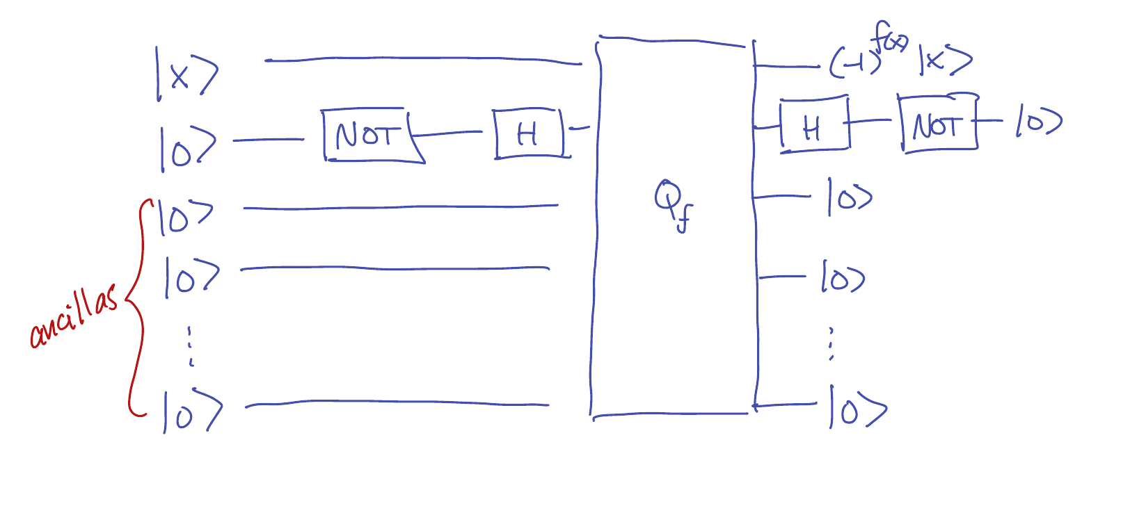
In other words, instead of taking \(y=0\) in \eqref{eq:standard}, we use \(y=\ket{-}\).
The result is:
\[Q_f : \ket{x} \ket{-} \ket{00 \cdots 0} \mapsto \ket{x} \frac{\ket{f(x)} - \ket{\neg f(x)}}{\sqrt{2}}
= (-1)^{f(x)} \ket{x} \ket{-} \ket{00 \cdots 0}.\]
Then after applying \(Q_f\), we apply a Hadamard gate followed by a NOT gate to transform \(\ket{-}\) into \(\ket{0}\).
-
The Bernstein-Vazirani problem: Here we are given a function \(f : \{0,1\}^n \to \{0,1\}\) and promised that
\[f(x) = \left(x_1 s_1 + x_2 s_2 + \cdots + x_n s_n\right) \bmod 2.\]
for some hidden vector \(s \in \{0,1\}^n\). The goal is to learn \(s\) by evaluating \(f\).
-
This can be done classically by using \(n\) queries, since \(f(e_1)=s_1,f(e_2)=s_2,\cdots,f(e_n)=s_n\),
where \(e_i\) is the vector with a \(1\) in the \(i\)th coordinate and zeros elsewhere.
And it is not hard to see that this is the smallest possible number of queries
that will always recover \(s\).
-
Here is a quantum circuit that evaluates \(f\) only once (with its input in superposition!) and outputs the
hidden vector \(s\) with certainty:
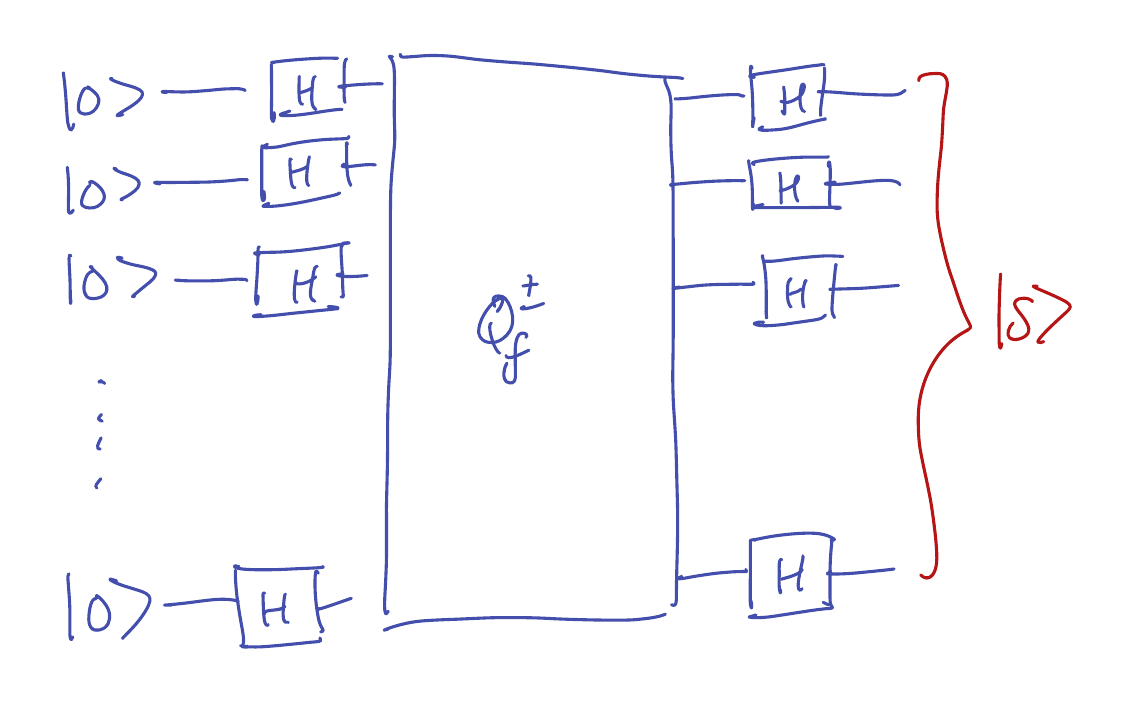
This output of the circuit can be summarized as \(H^{\otimes n} Q_f^{\pm} H^{\otimes n} \ket{00\cdots 0}\),
where \(H^{\otimes n} = H \otimes H \otimes \cdots \otimes H\) is an \(n\)-fold tensor product of Hadamard matrices,
and \(Q_f^{\pm}\) is a sign-implementation of \(f : \{0,1\}^n \to \{0,1\}\).
-
Analysis: After the first set of Hadamard gates, the overall state is
\[\begin{align*}
H^{\otimes n} \ket{00\cdots 0} &= (H \ket{0}) \otimes (H \ket{0}) \otimes \cdots \otimes (H \ket{0})
\\ &= \left(\frac{\ket{0}+\ket{1}}{\sqrt{2}}\right) \otimes \cdots \otimes \left(\frac{\ket{0}+\ket{1}}{\sqrt{2}}\right) \\
&= 2^{-n/2} \sum_{x \in \{0,1\}^n} \ket{x}.
\end{align*}\]
After applying \(Q_f^{\pm}\), the result is
\[\begin{equation}\label{eq:sup15}
2^{-n/2} \sum_{x \in \{0,1\}^n} (-1)^{f(x)} \ket{x}.
\end{equation}\]
To apply \(H^{\otimes n}\) to this state, it helps to observe that for \(x \in \{0,1\}^n\),
\[H^{\otimes n} \ket{x} = 2^{-n/2} \sum_{y \in \{0,1\}^n} \left(-1\right)^{x_1 y_1 + x_2 y_2 + \cdots + x_n y_n} \ket{y}.\]
Therefore applying \(H^{\otimes n}\) to \eqref{eq:sup15} gives
\[\begin{align}
2^{-n} \sum_{x,y \in \{0,1\}^n} (-1)^{f(x)} (-1)^{x_1 y_1 + \cdots + x_n y_n} \ket{y} &=
2^{-n} \sum_{x,y \in \{0,1\}^n} (-1)^{x_1 s_1 + \cdots + x_n s_n} (-1)^{x_1 y_1 + \cdots + x_n y_n} \ket{y} \nonumber \\
&=
2^{-n} \sum_{x,y \in \{0,1\}^n} (-1)^{x_1 (s_1+y_1) + \cdots + x_n (s_n+y_n)}\ket{y}. \label{eq:sup16}
\end{align}\]
Now note that for any fixed value of \(y\), we have
\[\sum_{x \in \{0,1\}^n} (-1)^{x_1 (s_1+y_1) + x_n (s_n+y_n)} = \begin{cases}
0 & y \neq s \\
1 & y = s.
\end{cases}\]
This equality holds because if \(s_i=y_i\), then \((s_i+y_i)\bmod 2 = 0\), and regardless of the value of \(x_i \in \{0,1\}\),
we have \((-1)^{x_i (s_i+y_i)} = 1\). On the other hand, if \(s_i \neq y_i\), then \((s_i+y_i)\bmod 2 = 1\),
and \((-1)^{x_i(s_i+y_i)} = (-1)^{x_i}\), meaning that the terms corresponding to \(x_i=0\) and \(x_i=1\) have
opposite signs and cancel out.
Therefore the output of the circuit \eqref{eq:sup16} is precisely \(\ket{s}\), revealing the hidden string \(s\).
|
Wed, Feb 09
Simon's algorithm
Suggested reading:
Mermin 2.5
|
Summary
-
Simon’s problem: Consider a function \(F : \{0,1\}^n \to \{0,1\}^m\) that is \(L\)-periodic in the
sense that for some \(L \in \{0,1\}^n\) with \(L \neq 00\cdots 0\), it holds that
\[F(x \oplus L) = F(x),\]
where \(x \oplus L\) is bitwise XOR, and moreover, we assume that \(F(x)=F(y) \iff y = x \oplus L\).
The problem is: Given access to a quantum circuit \(Q_F\) implementing \(F\), to determine \(L\)
using as few copies of \(Q_F\) as possible.
-
If we are only given a classical circuit \(C_F\) computing \(F\), it turns out this problem
is pretty difficult: At least \(\Omega(2^{n/2})\) copies of \(C_F\) are needed to build a probabilistic
circuit that recovers \(L\) with high probability.
-
Simon’s algorithm allows us to do this with a quantum algorithm that requires only \(4n\) copies of \(Q_F\),
an exponential improvement!
-
To accomplish this, we prepare the state
\[2^{-n/2} \sum_{x \in \{0,1\}^n} \ket{x} \ket{F(x)}.\]
-
Then we measure the qubits in the answer register. By definition of \(L\)-periodic, each possible value \(F(x)=y\)
occurs twice, since \(F(x)=F(x+L)=y\). The probability of measuring \(y\) is \(2^{-n+1}\), and then our state
collapses to
\[\frac{1}{\sqrt{2}} \left(\ket{x} \ket{y} + \ket{x+L} \ket{y}\right) =
\frac{1}{\sqrt{2}} \left(\ket{x} + \ket{x+L} \right) \otimes \ket{y}\]
-
After discarding the measured register (which is unentangled with the input register), we are left with the state
\(\frac{1}{\sqrt{2}} \left(\ket{x}+\ket{x+L}\right)\). Clearly if we knew both \(x\) and \(x+L\), then we could
take their bitwise XOR and recover \(L\).
-
Now we apply the Quantum Fourier transform again to this state, obtaining
\[\begin{align*}
H^{\otimes n} \frac{1}{\sqrt{2}} \left(\ket{x}+\ket{x+L}\right) &=
\frac{1}{\sqrt{2}}\left(2^{-n/2} \sum_{s \in \{0,1\}^n} (-1)^{x \cdot s} \ket{s} + 2^{-n/2}\sum_{s \in \{0,1\}^n} (-1)^{(x+L)\cdot s} \ket{s}\right)
\\
&=
2^{-(n+1)/2} \sum_{s \in \{0,1\}^n} (-1)^{x \cdot s} \left(1+(-1)^{L \cdot s}\right)\ket{s} \\
&= 2^{-(n-1)/2} \sum_{s : L \cdot s \bmod 2 = 0} (-1)^{x \cdot s} \ket{s}.
\end{align*}\]
-
When we measure this qubit, the outcome is a uniformly random string \(s \in \{0,1\}^n\) such that \(s \cdot L \bmod 2 = 0\).
-
Suppose we sample \(n-1\) such strings \(s^{(1)},s^{(2)},\ldots,s^{(n-1)}\) satisfying \(s^{(j)} \cdot L = 0\).
If these \(n-1\) vectors are linearly independent over \(\mathbb{F}_2\), then the system of linear equations
\[A = \begin{bmatrix} s^{(1)} \\ s^{(2)} \\ \vdots \\ s^{(n-1)} \end{bmatrix}, \quad A y = 0\]
has exactly two solutions (over \(\mathbb{F}_2\)): \(y=0\) and \(y=L\), and we can find the solution \(y=L\)
by (classical) Gaussian elimination.
-
Claim: With probability at least \(1/4\), it holds that \(s^{(1)},s^{(2)},\ldots,s^{(n-1)}\) are linearly
independent over \(\mathbb{F}_2\), meaning that with probability at least \(1/4\), we recover the hidden period \(L\).
-
Proof: If \(s^{(1)},\ldots,s^{(i)}\) are linearly independent, then they span
a \(2^i\)-dimensional subspace in \(\mathbb{F}_2^n\), which has \(2^i\) vectors, hence
\[\mathbb{P}\left[s^{(i+1)} \notin \mathrm{span}(s^{(1)},\ldots,s^{(i)})\right] = 1 - \frac{2^i}{2^n},\]
and
\[\begin{align*}
\mathbb{P}\left[s^{(1)},s^{(2)},\ldots,s^{(n-1)} \textrm{ linearly independent}\right] &=
\left(1-\frac{2^0}{2^n}\right) \left(1-\frac{2^1}{2^n}\right) \cdots \left(1-\frac{2^{(n-2)}}{2^n}\right)
\\
&\geq \frac12 \left(1-\frac{1}{4}-\frac{1}{8}-\cdots\right) \\
&= \frac{1}{4}\,.
\end{align*}\]
Related videos:
|
Mon, Feb 14
The quantum Fourier transform
Suggested reading:
N&C 5.1-5.2
|
Summary
-
The Quantum Fourier transform \(\mathbb{Z}_2^n\)
Define \(N \seteq 2^n\) and given \(g : \{0,1\}^n \to \mathbb{C}\) with \(\mathbb{E}_{x \in \{0,1\}^n} |g(x)|^2 = 1\),
encode \(g\) as the quantum state
\[\ket{g} \seteq \frac{1}{\sqrt{N}} \sum_{x \in \{0,1\}^n} g(x) \ket{x}.\]
Then applying \(H^{\otimes n}\) gives \(H^{\otimes n} \ket{g} = \sum_{s \in \{0,1\}^n} \hat{g}(s) \ket{s}\),
where
\[\hat{g}(s) = \mathbb{E}_{x \in \{0,1\}^n} g(x) (-1)^{s \cdot x}.\]
In other words, \(H^{\otimes n}\) implements the Fourier transform over \(\mathbb{Z}_2^n\).
Equivalently, \(H^{\otimes n}\) maps the Fourier basis \(\{ \ket{\chi_s} : s \in \{0,1\}^n \}\)
to the computational basis \(\{ \ket{x} : x \in \{0,1\}^n \}\), where
\(\chi_s(x) \seteq (-1)^{s \cdot x}\) and we similarly encode
\[\ket{\chi_s} = \frac{1}{\sqrt{N}} \sum_{x \in \{0,1\}^n} \chi_S(x) \ket{x}.\]
In this notation, we can write \(\hat{g}(s) = \ip{\chi_s}{g}\).
-
The Quantum Fourier transform over \(\mathbb{Z}_N\)
We use \(\mathbb{Z}_N\) to denote the integers modulo \(N\). Given \(g : \mathbb{Z}_N \to \mathbb{C}\) with
\(\mathbb{E}_{x \in \mathbb{Z}_N} |g(x)|^2 = 1\), we can similarly encode \(g\) as a quantum state:
\[\ket{g} \seteq \frac{1}{\sqrt{N}} \sum_{x \in \mathbb{Z}_N} g(x) \ket{x}.\]
Now the Fourier basis is given by the functions
\[\chi_s(x) \seteq \omega_N^{s x}, \quad s \in \mathbb{Z}_N,\]
where \(\omega_N \seteq e^{2\pi i/N}\) is a primitive \(N\)th root of unity.
These functions can similarly be encoded as quantum states:
\[\ket{\chi_s} \seteq \frac{1}{\sqrt{N}} \sum_{x \in \mathbb{Z}_n} \chi_s(x) \ket{x}.\]
You should verify that the vectors \(\{ \ket{\chi_s} : s \in \mathbb{Z}_N \}\) actually form
an orthonormal basis of \(\mathbb{C}^N\).
The quantum Fourier transform is given by the unitary map
\[\ket{g} \mapsto \sum_{s \in \mathbb{Z}_N} \ip{\chi_s}{g} \ket{s} = \sum_{s \in \mathbb{Z}_N} \left(\mathbb{E}_{x \in \mathbb{Z}_N} \left[\omega_N^{-sx} g(x)\right]\right)\ket{s},\]
where we have used the fact that the complex conjugate of \(\omega_N\) is \(\bar{\omega}_N = \omega_N^{-1} = e^{-2\pi i/N}\).
-
An efficient implementation of the quantum Fourier transform over \(\mathbb{Z}_N\)
Assume now that \(N = 2^n\) for some \(n \geq 1\) and define \(\omega \seteq \omega_N = e^{2\pi i/N}\).
The Fourier transform over \(\mathbb{Z}_2^n\) could be implemented using only \(O(n)\) quantum gates.
A related implementation is possible over \(\mathbb{Z}_N\). We need to implement the unitary change of basis:
\[\mathsf{DFT}_N \ket{x} = \sum_{s \in \mathbb{Z}_N} \ip{\chi_s}{x} \ket{s}.\]
Let us write in binary \(x = x_{n-1} x_{n-2} \cdots x_1 x_0\). Then we have
\[\mathsf{DFT}_N \ket{x} = \frac{1}{\sqrt{N}} \sum_{s \in \mathbb{Z}_N} \bar{\omega}^{s x} \ket{s},\]
and we can write this as the tensor product
\[\left(\frac{\ket{0} + \bar{\omega}^{2^{n-1} x_{n-1}} \ket{1}}{\sqrt{2}}\right) \otimes
\left(\frac{\ket{0} + \bar{\omega}^{2^{n-2} x_{n-2}} \ket{1}}{\sqrt{2}}\right) \otimes \cdots \otimes
\left(\frac{\ket{0} + \bar{\omega}^{2 x_1} \ket{1}}{\sqrt{2}}\right) \otimes
\left(\frac{\ket{0} + \bar{\omega}^{x_0} \ket{1}}{\sqrt{2}}\right).\]
Let us write this as \(\ket{s_{n-1}} \otimes \ket{s_{n-2}} \otimes \cdots \otimes \ket{s_1} \otimes \ket{s_0}\),
and then it suffices to produce a circuit where the output wires carry each \(\ket{s_j}\).
-
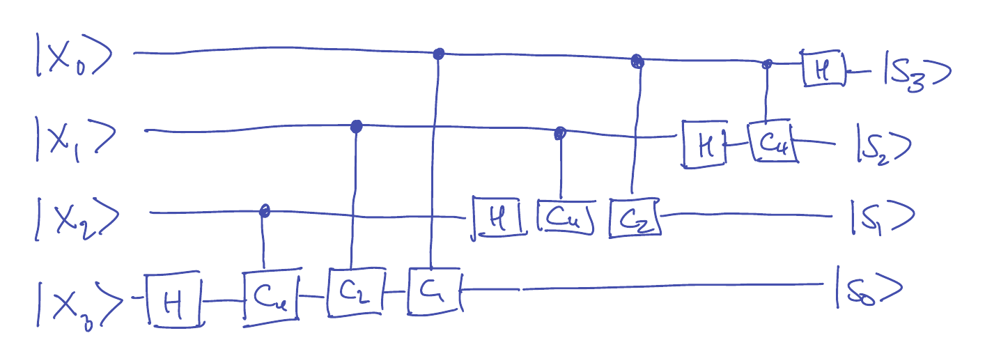
The case \(N=16\). It is instructive to do this for a fixed value, say \(N=16\). Then we have
\[\begin{align*}
\mathsf{DFT}_{16} \ket{x}
&=
\frac{1}{4} \left(\ket{0000} + \bar{\omega}^{x} \ket{0001} + \bar{\omega}^{2x} \ket{0010} + \bar{\omega}^{3x} \ket{0011} + \cdots + \bar{\omega}^{15x} \ket{1111}\right) \\
&=
\left(\frac{\ket{0} + \bar{\omega}^{8 x} \ket{1}}{\sqrt{2}}\right) \otimes
\left(\frac{\ket{0} + \bar{\omega}^{4 x} \ket{1}}{\sqrt{2}}\right) \otimes
\left(\frac{\ket{0} + \bar{\omega}^{2 x} \ket{1}}{\sqrt{2}}\right) \otimes
\left(\frac{\ket{0} + \bar{\omega}^{x} \ket{1}}{\sqrt{2}}\right) \\
&= \ket{s_3} \otimes \ket{s_2} \otimes \ket{s_1} \otimes \ket{s_0},
\end{align*}\]
where in the last line we are just giving names to each piece of the tensor product
that we would like to produce on the output wires.
Starting with \(\ket{s_3}\), we have
\[\bar{\omega}^{8x} = \bar{\omega}^{8 (8x_3 + 4x_2 + 2x_1 + x_0)} = \bar{\omega}^{8 x_0},\]
since the other terms in the exponent vanish modulo 16.
Note that \(\bar{\omega}^8 = -1\), hence we have
\[\ket{s_3} = \frac{\ket{0} + (-1)^{x_0}\ket{1}}{\sqrt{2}} = H \ket{x_0}.\]
Similarly, we have
\[\bar{\omega}^{4x} = \bar{\omega}^{8x_1} \bar{\omega}^{4x_0} = (-1)^{x_1} \bar{\omega}^{4 x_0},\]
so we can write
\[\ket{s_2} = \frac{\ket{0} + (-1)^{x_1} \bar{\omega}^{4 x_0} \ket{1}}{\sqrt{2}}\]
Let \(\mathsf{C}_{4}\) be a \(2\)-qubit “controlled \(\bar{\omega}^4\) gate”
in the sense that
\[\begin{align*}
\mathsf{C}_{4} \ket{0} \ket{b} &= \ket{0} \ket{b}, \\
\mathsf{C}_4 \ket{1} \ket{0} &= \ket{1} \ket{0} \\
\mathsf{C}_4 \ket{1} \ket{1} &= \ket{1} \bar{\omega}^4 \ket{1}.
\end{align*}\]
Note that this is specified by the \(4 \times 4\) matrix
\[\mathsf{C}_4 = \begin{bmatrix} 1 & 0 & 0 & 0 \\ 0 & 1 & 0 & 0 \\ 0 & 0 & 1 & 0 \\ 0 & 0 & 0 & \bar{\omega}^4 \end{bmatrix}.\]
Then we can write (check this!):
\[\ket{s_2} = \mathsf{C}_4 \ket{x_0} H \ket{x_1}.\]
Continuing this way yields a circuit for all \(4\) output wires:
-
In the general case, the number of gates needed is \(1+2+\cdots+(n-1)+n \leq \frac{n(n+1)}{2}\).
If one wants to implement the circuit approximately (but sufficient, e.g., for Shor’s algorithm),
it is possible to use only \(O(n \log n)\) \(1\)- and \(2\)-qubit gates.
Related videos:
|
Wed, Feb 16
Shor's algorithm I: Period finding
Suggested reading:
N&C 5.3
|
Summary
- Consider \(N=2^n\) and let \(\mathbb{Z}_N\) denote the integers modulo \(N\).
-
Suppose we have a function \(F : \mathbb{Z}_N \to \{1,\ldots,M\}\) that is \(L\)-periodic in the sense that
\[F(x)=F(y) \iff L \mid x-y,\]
and our goal is to find the period $L$.
-
Recall that we assume \(F\) is implemented by a circuit with the behavior:
\[Q_F : \ket{x} \ket{y} \mapsto \ket{x} \ket{y \oplus F(x)}.\]
-
We will use a variant of Simon’s algorithm, as follows:
-
First we prepare the state
\[Q_F (H^{\otimes n} \ket{00\cdots 0}) \ket{00 \cdots 0} \frac{1}{\sqrt{N}} = \sum_{x \in \mathbb{Z}_N} \ket{x} \ket{F(x)},\]
-
Then we measure the second register, obtaining an outcome \(c^* \in \{1,\ldots,M\}\), and the state collapses to
\[\sqrt{\frac{1}{L}}\sum_{x : F(x)=c^*} \ket{x}\ket{c^*}.\]
Note that since \(F\) has period \(L\), it must be that \(L\) divides \(N\) and the number of colors used is \(L\),
and each color is used \(M=N/L\) times. So we see each
\(c^* \in \{1,\ldots,M\}\) with probability \(1/M = L/N\).
-
Finally, we discard the second register (note that it is unentangled with the first register), yielding the state
\[\ket{g_{c^*}} = \sum_{x \in \mathbb{Z}_N} g_{c^*}(x),\]
where \(g_{c^*} : \mathbb{Z}_N \to \mathbb{C}\) is given by
\[g_{c^*}(x) = \begin{cases}
\sqrt{L} & F(x)=c^* \\
0 & \textrm{otherwise.}
\end{cases}\]
-
Now we use the Quantum Fourier transform from the previous lecture to compute
\[\mathsf{DFT}_N \ket{g_{c^*}} = \sum_{s=0}^{N-1} \hat{g}_{c^*}(s) \ket{s},\]
and we measure the register, yielding the measurement outcome \(s\) with probability \(\mag{\hat{g}_{c^*}(s)}^2\).
-
Computing the Fourier transform yields
\[\mag{\hat{g}_{c^*}(s)}^2 = \frac{M}{N} \mathbf{1}_{\{0,M,2M,3M,\ldots,N-M\}}(s).\]
In other words, the outcome of the measurement is a uniformly random number \(s \in \{0,M,2M,3M,\ldots,N-M\}\), i.e., a random multiple of \(M\).
Note that from \(M\) we can compute \(L=N/M\).
By running the whole algorithm twice, we find two random multiples \(k_1 M\) and \(k_2 M\), and it holds that
\[\Pr[\gcd(k_1 M, k_2 M)=M] \geq \frac1{12},\]
thus with constant probability we recover \(M\), from which we can compute the period \(L\).
-
This still works even if we only assume that \(F\) is almost \(L\)-periodic in the sense that
\[F(x)=F(y) \iff y=x+k\cdot L, k \geq 0.\]
where now addition is not taken modulo \(N\) (so it is not required that \(L\) divides \(N\)).
In this case, Fourier sampling has the following guarantee: With probability at least \(2/5\), we see
\(\closeint{k \frac{N}{L}}\) where \(k \in \{0,1,\ldots,L-1\}\) is chosen uniformly at random,
and \(\closeint{x}\) denotes the closest integer to \(x\).
|
Wed, Feb 23
Shor's algorithm II: Factoring
Suggested reading:
N&C 5.3-5.4
|
Summary
- We show how period-finding leads to an algorithm for factoring. The reduction is entirely classical.
- Suppose \(p,q\) are distinct prime numbers and \(B=pq\). Given an \(m\)-bit number \(B\) as input, we want to find \(p\) and \(q\).
- To do this, we saw that it suffices to find a non-trivial square-root of \(1\) modulo \(B\).
- On Homework #4, you will show that the following works with probability \(1/2\):
- Choose \(a \in \mathbb{Z}_B^*\) uniformly at random.
- Define \(F : \mathbb{Z}_N \to \mathbb{Z}_N\) by \(F(x) \seteq a^x \bmod B\), where we take \(N=2^n\) and \(n \seteq 10 m\).
- If \(L \seteq \mathrm{ord}_{\mathbb{Z}_B^*}(a)\) is the order of \(a\) modulo \(B\), then
\(F\) will be almost \(L\)-periodic.
- Now we use the quantum period-finding algorithm from the previous lecture to find \(L\).
- If \(L\) is even, then our candidate for a non-trivial square-root of \(1\) is the number \(a^{L/2}\).
On the homework, you will show that with probability at least \(1/2\), it
holds that \(L\) is even and \(a^{L/2} \neq \pm 1 \bmod B\).
-
The last part of the lecture was devoted to finding \(L\) in the case when the function \(F\) is almost \(L\)-periodic.
(We saw how to do this already when \(F\) is exactly \(L\)-periodic.)
Recall that in this case, with probability at least \(2/5\), we obtain \(s \seteq \closeint{k \frac{N}{L}}\) for
a uniformly random \(k \in \{0,1,\ldots,L-1\}\).
-
Therefore we have
\[\frac{s}{N} \approx \frac{k}{L} \pm \frac{0.5}{N}\]
for some integer \(k\).
Now we construct the continued fraction expansionof \(s/N\),
which produces a sequence of approximations to \(s/N\).
Lemma: If \(|\frac{s}{N}-\frac{k}{L}| \leq \frac{1}{2L^2}\), then \(k/L\) occurs as one of the
convergents in the continued fraction expansion of \(s/N\).
This is why we choose \(N = 2^{n}\) where \(n = 10 m\), to ensure that \(0.5/N \leq 1/(2L^2)\) (with room to spare).
- So we get the fraction \(k/L\) in lowest terms. If \(\gcd(k,L)=1\), then we can use that to recover \(L\).
Since \(k \in \{0,1,\ldots,L-1\}\) is uniformly random, it will be prime with probability at least \(\Omega(1/\log(L))\)
by the Prime Number Theorem.
|
Mon, Feb 28
Grover's algorithm
Suggested reading:
N&C 6.1-6.2
|
Summary
- Given a function \(F : \{0,1\}^n \to \{0,1\}\), we would like to find an \(x \in \{0,1\}^n\) such that \(F(x)=1\).
-
Recall that \(Q_F^{\pm}\) is the sign oracle implementation of \(F\), where
\[Q_F^{\pm} \ket{x} = (-1)^{F(x)} \ket{x},\qquad x \in \{0,1\}^n.\]
-
The Grover iteration is given by the unitary
\(G \seteq (2 \ket{\psi}\bra{\psi} - I) Q_F^{\pm},\)
where \(\ket{\psi} \seteq \frac{1}{\sqrt{N}} \sum_{x \in \{0,1\}^n} \ket{x}\).
You should check that \(2 \ket{\psi}\bra{\psi} - I\) is a unitary matrix, and that it can be efficiently
implemented on a quantum computer because
\[2 \ket{\psi}\bra{\psi} - I = H^{\otimes n} Q_{\mathrm{OR}}^{\pm 1} H^{\otimes n},\]
where \(Q_{\mathrm{OR}}^{\pm 1}\) is defined by \(\ket{x} \mapsto (-1)^{\mathrm{OR}(x)} \ket{x}\) for \(x \in \{0,1\}^n\).
-
Define \(M = \mag{\{ x : F(x) = 1 \}}\) and the states
\[\begin{align*}
\ket{\alpha} &\seteq \frac{1}{\sqrt{M}} \sum_{x : F(x)=1} \ket{x} \\
\ket{\beta} &\seteq \frac{1}{\sqrt{N-M}} \sum_{x : F(x)=0} \ket{x}.
\end{align*}\]
Then we can write the uniform superposition as
\[\ket{\psi} = \sqrt{\frac{M}{N}} \ket{\alpha} + \sqrt{\frac{N-M}{N}} \ket{\beta}.\]
-
It turn outs that \(G \ket{\psi}\) remains in the plane spanned by \(\{\ket{\alpha},\ket{\beta}\}\), so this is
also true for \(G^k \ket{\psi}\) for all \(k \geq 1\).
This is true because
\[Q_F^{\pm} \left(a \ket{\alpha} + b \ket{\beta}\right) = -a \ket{\alpha} + b \ket{\beta},\]
hence \(Q_F^{\pm}\) is a reflection around the \(\ket{\beta}\) axis (in the \(\ket{\alpha},\ket{\beta}\) plane).
Moreover,
\[(2 \ket{\psi}\bra{\psi} - I) (c_0 \ket{\psi} + c_1 \ket{\psi^{\perp}}) = c_0 \ket{\psi} - c_1 \ket{\psi^{\perp}},\]
for any vector \(\ket{\psi^{\perp}}\) that is orthogonal to \(\ket{\psi}\), so this operator is a reflection about \(\ket{\psi}\).
-
We conclude that \(G\) maps the \(\{\ket{\alpha},\ket{\beta}\}\) plane to itself and is the composition of two reflections.
That means \(G\) is rotation, and we can calculate that if
\[\ket{\psi} = \cos(\theta) \ket{\beta} + \sin(\theta) \ket{\alpha},\]
then
\[G \ket{\psi} = \cos(3\theta) \ket{\beta} + \sin(3\theta) \ket{\alpha},\]
hence in the \(\{\ket{\alpha},\ket{\beta}\}\) plane, \(G\) is a rotation by angle \(2\theta\). Therefore:
\[G^k \ket{\psi} = \cos ((2k+1)\theta) \ket{\beta} + \sin ((2k+1)\theta) \ket{\alpha}\]
-
Since \(\cos(\epsilon) = 1 - \frac12 \epsilon^2 + O(\epsilon^4)\),
it holds that for \(M \leq N/2\), we have \(\theta \approx \sqrt{M/N}\).
Hence we can choose \(k \leq O(\sqrt{M/N})\) appropriately so that
\[\sin((2k+1)\theta) \geq 0.1,\]
in which case, when we measure, we have at least a 10% chance of sampling an \(x\) such that \(F(x)=1\).
-
We can accomplish this even if we only know that \(M \in [2^{-j} N, 2^{-j+1} N)\) for some \(j\).
Hence we can try \(j=1,2,3,\ldots\) until we find an \(x\) such that \(F(x)=1\). The number of queries we need
will be on the order of
\[\sqrt{2^1} + \sqrt{2^2} + \cdots + \sqrt{2^j} \leq O\left(\sqrt{N/M}\right).\]
|
| Quantum information theory |
Wed, Mar 02
Quantum probability
|
Lecture notes from The art and science of PSD matrices:
|
Mon, Mar 07
Quantum information
|
Lecture notes from The art and science of PSD matrices:
|
Wed, Mar 09
Partial trace and the Holevo bound
|
|